The Science of Doom

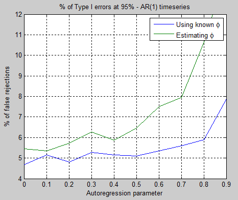
In the last article we saw some testing of the simplest autoregressive model AR(1). I still have an outstanding issue raised by one commenter relating to the hypothesis testing that was introduced, and I hope to come back to it at a later stage.

Different Noise Types

Before we move onto more general AR models, I did do some testing of the effectiveness of the hypothesis test for AR(1) models with different noise types.

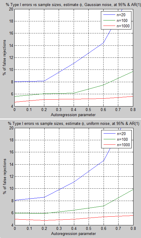
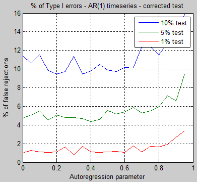
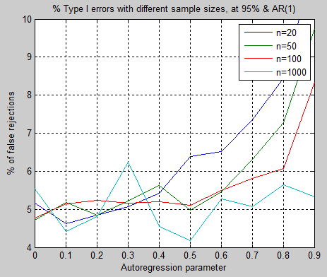
The testing shown in Part Four has Gaussian noise (a “normal distribution”), and the theory applied is only apparently valid for Gaussian noise, so I tried uniform distribution of noise and also a Gamma noise distribution:

Figure 1

The Gaussian and uniform distribution produce the same results. The Gamma noise result isn’t shown because it was also the same.

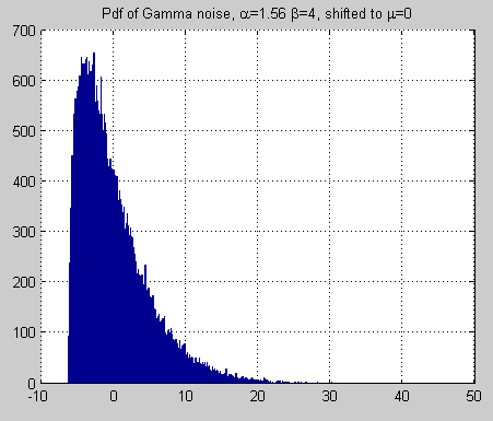
A Gamma distribution can be quite skewed, which was why I tried it – here is the Gamma distribution that was used (with the same variance as the Gaussian, and shifted to produce the same mean = 0):

Figure 2

So in essence I have found that the tests work just as well when the noise component is uniformly distributed or Gamma distributed as when it has a Gaussian distribution (normal distribution).

Hypothesis Testing of AR(1) Model When the Model is Actually AR(2)

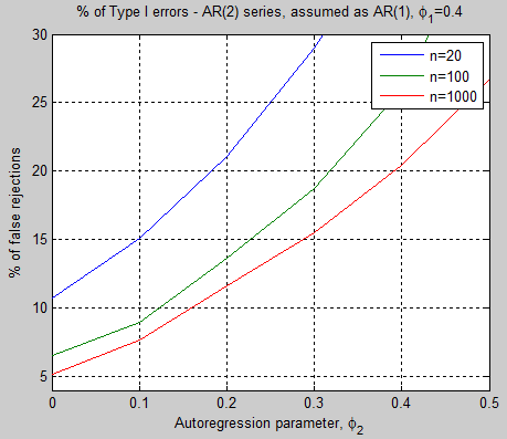
The next idea I was interested to try was to apply the hypothesis testing from Part Three on an AR(2) model, when we assume incorrectly that it is an AR(1) model.

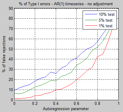
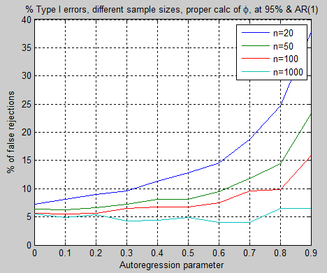
Remember that the hypothesis test is quite simple – we produce a series with a known mean, extract a sample, and then using the sample find out how many times the test rejects the hypothesis that the mean is different from its actual value:

Figure 3

As we can see, the test, which should be only rejecting 5% of the tests, rejects a much higher proportion as φ₂ increases. This simple test is just by way of introduction.

Higher Order AR Series

The AR(1) model is very simple. As we saw in Part Three, it can be written as:

x_t – μ = φ(x_t-1 – μ) + ε_t

where x_t = the next value in the sequence, x_t-1 = the last value in the sequence, μ = the mean, ε_t = random quantity and φ = auto-regression parameter

[Minor note, the notation is changed slightly from the earlier article]

In non-technical terms, the next value in the series is made up of a random element plus a dependence on the last value – with the strength of this dependence being the parameter φ.

The more general autoregressive model of order p, AR(p), can be written as:

x_t – μ = φ₁(x_t-1 – μ) + φ₂(x_t-2 – μ) + .. + φ_p(x_t-p – μ) + ε_t

φ₁..φ_p = the series of auto-regression parameters

In non-technical terms, the next value in the series is made up of a random element plus a dependence on the last few values. So of course, the challenge is to determine the order p, and then the parameters φ₁..φ_p

There is a bewildering array of tests that can be applied, so I started simply. With some basic algebraic manipulation (not shown – but if anyone is interested I will provide more details in the comments), we can produce a series of linear equations known as the Yule-Walker equations, which allow us to calculate φ₁..φ_p from the estimates of the autoregression.

If you look back to Figure 2 in Part Three you see that by regressing the time series with itself moved by k time steps we can calculate the lag-k correlation, r_k, for k=1, 2, 3, etc. So we estimate r₁, r₂, r₃, etc., from the sample of data that we have, and then solve the Yule-Walker equations to get φ₁..φ_p

First of all I played around with simple AR(2) models. The results below are for two different sample sizes.

A population of 90,000 is created (actually 100,000 then the first 10% is deleted), and then a sample is randomly selected 10,000 times from this population. For each sample, the Yule-Walker equations are solved (each of 10,000 times) and then the results are averaged.

In these results I normalized the mean and standard deviation of the parameters by the original values (later I decided that made it harder to see what was going on and reverted to just displaying the actual sample mean and sample standard deviation):

Figure 4

Notice that the sample size of 1,000 produces very accurate results in the estimation of φ₁ & φ₂, with a small spread. The sample size of 50 appears to produce a low bias in the calculated results, especially for φ₂, which is no doubt due to not reading the small print somewhere..

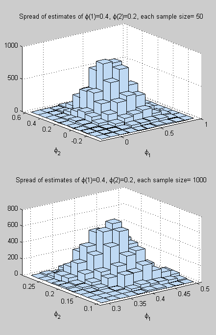
Here is a histogram of the results, showing the spread across φ₁ & φ₂ – note the values on the axes, the sample size of 1000 produces a much tighter set of results, the sample size of 50 has a much wider spread:

Figure 5

Then I played around with a more general model. With this model I send in AR parameters to create the population, but can define a higher order of AR to test against, to see how well the algorithm estimates the AR parameters from the samples.

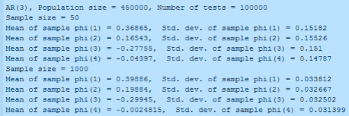
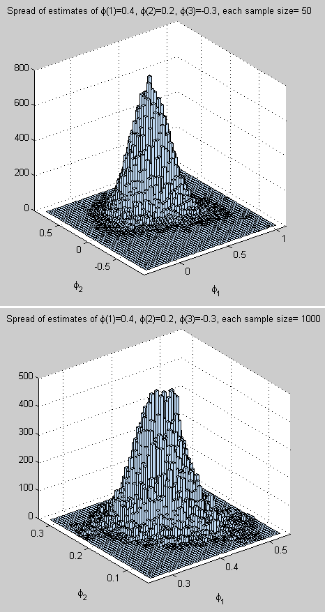
In the example below the population is created as AR(3), but tested as if it might be an AR(4) model. The AR(3) parameters (shown on the histogram in the figure below) are φ₁= 0.4, φ₂= 0.2, φ₃= -0.3.

The estimation seems to cope quite well as φ₄ is estimated at about zero:

Figure 6

The histogram of results for the first two parameters, note again the difference in values on the axes for the different sample sizes:

Figure 7

[The reason for the finer detail on this histogram compared with figure 5 is just discovery of the Matlab parameters for 3d histograms].

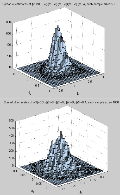
Rotating the histograms around in 3d appears to confirm a bell-curve. Something to test formally at a later stage.

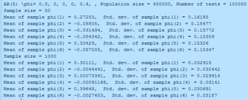
Here’s an example of a process which is AR(5) with φ₁= 0.3, φ₂= 0, φ₃= 0, φ₄= 0, φ₅= 0.4; tested against AR(6):

Figure 8

And the histogram of estimates of φ₁& φ₂:

Figure 8

ARMA

We haven’t yet seen ARMA models – auto-regressive moving average models. And we haven’t seen MA models – moving average models with no auto-regressive behavior.

What is an MA or “moving average” model?

The term in the moving average is a “linear filter” on the random elements of the process. So instead of ε_t as the “uncorrelated noise” in the AR model we have ε_t plus a weighted sum of earlier random elements. The MA process, of order q, can be written as:

x_t – μ = ε_t + θ₁ε_t-1+ θ₂ε_t-2 + .. + θ_pε_t-p

θ₁..θ_p = the series of moving average parameters

The term “moving average” is a little misleading, as Box and Jenkins also comment.

Why is it misleading?

Because for AR (auto-regressive) and MA (moving average) and ARMA (auto-regressive moving average = combination of AR & MA) models the process is stationary.

This means, in non-technical terms, that the mean of the process is constant through time. That doesn’t sound like “moving average”.

So think of “moving average” as a moving average (filter) of the random elements, or noise, in the process. By their nature these will average out over time (because if the average of the random elements = 0, the average of the moving average of the random elements = 0).

An example of this in the real world might be a chemical introduced randomly into a physical process  – this is the ε_t term – but because the chemical gets caught up in pipework and valves, the actual value of the chemical released into the process at time t is the sum of a proportion of the current value released plus a proportion of earlier values released. Examples of the terminology used for the various processes:

• AR(3) is an autoregressive process of order 3
• MA(2) is a moving average process of order 2
• ARMA(1,1) is a combination of AR(1) and MA(1)

References

Time Series Analysis: Forecasting & Control, 3rd Edition, Box, Jenkins & Reinsel, Prentice Hall (1994)

Read Full Post »

In Part Three we started looking at time-series that are autocorrelated, which means each value has a relationship to one or more previous values in the time-series. This is unlike the simple statistical models of independent events.

And in Part Two we have seen how to test whether a sample comes from a population of a stated mean value. The ability to run this test is important and in Part Two the test took place for a population of independent events.

The theory that allows us to accept or reject hypotheses to a certain statistical significance does not work properly with serially correlated data (not without modification).

Here is a nice example from Wilks:

Figure 1

Remember that (usually) with statistical test we don’t actually know the whole population – that’s what we want to find out about. Instead, we take a sample and attempt to find out information about the population.

Take a look at figure 1 – the lighter short horizontal lines are the means (the “averages”) of a number of samples. If you compare the top and bottom graphs you see that the distribution of the means of samples is larger in the bottom graph. This bottom graph is the timeseries with autocorrelation.

What this means is that if we take a sample from a time-series and apply the standard Student-t test to find out whether it came from a population of mean = μ, we will calculate that it didn’t come from a mean that it actually did come from too many times. So a 95% test will incorrectly reject the hypothesis a lot more than 5%.

To demonstrate this, here is the % of false rejections (“Type I errors”) as the autocorrelation parameter increases, when a standard Student-t test is applied:

Figure 2

The test was done with Matlab, with a time-series population of 100,000, Gaussian (“normal distribution”) errors, and samples of 100 taken 10,000 times (in each case a random start point was chosen then the next 100 points were taken as a sample – this was repeated 10,000 times). When the time-series is generated with no serial correlation, the hypothesis test works just fine. As the autocorrelation increases (as we move to the right of the graph), the hypothesis test starts creating more false fails.

With AR(1) autocorrelation – the simplest model of autocorrelation – there is a simple correction that we can apply. This goes under different names like effective sample size and variance inflation factor.

For those who like details, instead of the standard deviation of the sample means:

s = σ/√n

we derive:

s = σ.√[(1+ρ)/n.(1-ρ)], where ρ = autocorrelation parameter.

Repeating the same test with the adjusted value:

Figure 3

We see that Type I errors start to get above our expected values at higher values of autocorrelation. (I’m not sure whether that actually happens with an infinite number of tests and true random samples).

Note as well that the tests above were done using the known value of the autocorrelation parameter (this is like having secret information which we don’t normally have).

So I re-ran the tests using the derived autocorrelation parameter from the sample data (regressing the time-series against the same time-series with a one time step lag) – and got similar, but not identical results and apparently more false fails.

Curiosity made me continue (tempered by the knowledge of the large time-wasting exercise I had previously engaged in because of a misplaced bracket in one equation), so I rewrote the Matlab program to allow me to test some ideas a little further. It was good to rewrite because I was also wondering whether having one (long) time-series generated with lots of tests against it was as good as repeatedly generating a time-series and carrying out lots of tests each time.

So this following comparison had a time-series population of 100,000 events, samples of 100 items for each test, repeated for 100 tests, then the time-series regenerated – and this done 100 times. So 10,000 tests across 100 different populations – first with the known autoregression parameter, then with the estimated value of this parameter from the sample in question:

Figure 4 – Each sample size = 100

The correct value of rejected tests should be 5% no matter what the autoregression parameter.

The rewritten program allows us to test for the effect of sample size. The following graph uses the known value of autogression parameter in the test, a time-series population of 100,000, drawing samples out 1000 times from each population, and repeating through 10 populations in total:

Figure 5 – Using known value of autoregression parameter in Student T-test

Remembering that all of the lines should be horizontal on 5%, we can see that the largest sample population of 1000 is the most resistant to higher autoregression parameters.

This reminded me that the equation for the variance inflation factor (shown earlier) is in fact an approximation. The correct formula (for those who like to see such things):

Figure 6

So I adjusted the variance inflation factor in the program and reran.

I’m really starting to slow things down now – because in each single hypothesis test we are estimating the autoregression parameter, ρ, by a lag-1 correlation, then with this estimate we have to calculate the above circled formula, which requires summing the equation from 1 through to the number of samples. So in the case of n=1000 that’s 1000 calculations, all summed, then used in a Student-t test. And this is done in each case for 1000 tests per population x 10 populations.. thank goodness for Matlab which did it in 18 minutes. (And apologies to readers trying to follow the detail – in the graphics I show the autoregression parameter as φ, when I meant to use ρ, no idea why..)

Fortunately, the result turns out almost identical to using the approximation (the graph using the approximation is not shown):

Figure 7 – Using estimated autoregression parameter

So unless I have made some kind of mistake (quite possible), I take this to mean that the sampling uncertainty in the autoregression parameter adds uncertainty to the Student T-test, which can’t be corrected for easily.

With large samples, like 1000, it appears to work just fine. With time-series data from the climate system we have to take what we can get and mostly it’s not 1000 points.

We are still considering a very basic model – AR(1) with normally-distributed noise.

In the next article I hope to cover some more complex models, as well as the results from this kind of significance test if we assume AR(1) with normally-distributed noise yet actually have a different model in operation..

References

Statistical Methods in the Atmospheric Sciences, 3rd edition, Daniel Wilks, Academic Press (2011)

Taking Serial Correlation into Account in Tests of the Mean, Zwiers & von Storch, Journal of Climate (1995)

Read Full Post »