In the last article we looked at a paper which tried to unravel – for clear sky only – how the OLR (outgoing longwave radiation) changed with surface temperature. It did the comparison by region, by season and from year to year.
The key point for new readers to understand – why are we interested in how OLR changes with surface temperature? The concept is not so difficult. The practical analysis presents more problems.
Let’s review the concept – and for more background please read at least the start of the last article: if we increase the surface temperature, perhaps due to increases in GHGs, but it could be due to any reason, what happens to outgoing longwave radiation? Obviously, we expect OLR to increase. The real question is how by how much?
If there is no feedback then OLR should increase by about 3.6 W/m² for every 1K in surface temperature (these values are global averages):
- If there is positive feedback, perhaps due to more humidity, then we expect OLR to increase by less than 3.6 W/m² – think “not enough heat got out to get things back to normal”
- If there is negative feedback, then we expect OLR to increase by more than 3.6 W/m². In the paper we reviewed in the last article the authors found about 2 W/m² per 1K increase – a positive feedback, but were only considering clear sky areas
One reader asked about an outlier point on the regression slope and whether it affected the result. This motivated me to do something I have had on my list for a while now – get “all of the data” and analyse it. This way, we can review it and answer questions ourselves – like in the Visualizing Atmospheric Radiation series where we created an atmospheric radiation model (first principles physics) and used the detailed line by line absorption data from the HITRAN database to calculate how this change and that change affected the surface downward radiation (“back radiation”) and the top of atmosphere OLR.
With the raw surface temperature, OLR and humidity data “in hand” we can ask whatever questions we like and answer these questions ourselves..
NCAR reanalysis, CERES and AIRS
CERES and AIRS – satellite instruments – are explained in CERES, AIRS, Outgoing Longwave Radiation & El Nino.
CERES measures total OLR in a 1ºx 1º grid on a daily basis.
AIRS has a “hyper-spectral” instrument, which means it looks at lots of frequency channels. The intensity of radiation at these many wavelengths can be converted, via calculation, into measurements of atmospheric temperature at different heights, water vapor concentration at different heights, CO2 concentration, and concentration of various other GHGs. Additionally, AIRS calculates total OLR (it doesn’t measure it – i.e. it doesn’t have a measurement device from 4μm – 100μm). It also measures parameters like “skin temperature” in some locations and calculates the same in other locations.
For the purposes of this article, I haven’t yet dug into the “how” and the reliability of surface AIRS measurements. The main point to note about satellites is they sit at the “top of atmosphere” and their ability to measure stuff near the surface depends on clever ideas and is often subverted by factors including clouds and surface emissivity. (AIRS has microwave instruments specifically to independently measure surface temperature even in cloudy conditions, because of this problem).
NCAR is a “reanalysis product”. It is not measurement, but it is “informed by measurement”. It is part measurement, part model. Where there is reliable data measurement over a good portion of the globe the reanalysis is usually pretty reliable – only being suspect at the times when new measurement systems come on line (so trends/comparisons over long time periods are problematic). Where there is little reliable measurement the reanalysis depends on the model (using other parameters to allow calculation of the missing parameters).
Some more explanation in Water Vapor Trends under the sub-heading Reanalysis – or Filling in the Blanks.
For surface temperature measurements reanalysis is not subverted by models too much. However, the mainstream surface temperature series are surely better than NCAR – I know that there is an army of “climate interested people” who follow this subject very closely. (I am not in that group).
I used NCAR because it is simple to download and extract. And I expect – but haven’t yet verified – that it will be quite close to the various mainstream surface temperature series. If someone is interested and can provide daily global temperature from another surface temperature series as an Excel, csv, .nc – or pretty much any data format – we can run the same analysis.
For those interested, see note 1 on accessing the data.
Results – Global Averages
For our starting point in this article I decided to look at global averages from 2001 to 2013 inclusive (data from CERES not yet available for the whole of 2014). This was after:
- looking at daily AIRS data
- creating and comparing NCAR over 8 days with AIRS 8-day averages for surface skin temperature and surface air temperature
- creating and comparing AIRS over 8-days with CERES for TOA OLR
More on those points in later articles.
The global relationship with surface temperature and OLR is what we have a primary interest in – for the purpose of determining feedbacks. Then we want to figure out some detail about why it occurs. I am especially interested in the AIRS data because it is the only global measurement of upper tropospheric water vapor (UTWV) – and UTWV along with clouds are the key factors in the question of feedback – how OLR changes with surface temperature. For now, we will look at the simple relationship between surface temperature (“skin temperature”) and OLR.
Here is the data, shown as an anomaly from the global mean values over the period Jan 1st, 2001 to Dec 31st, 2013. Each graph represents a different lag – how does global OLR (CERES) change with global surface temperature (NCAR) on a lag of 1 day, 7 days, 14 days and so on:
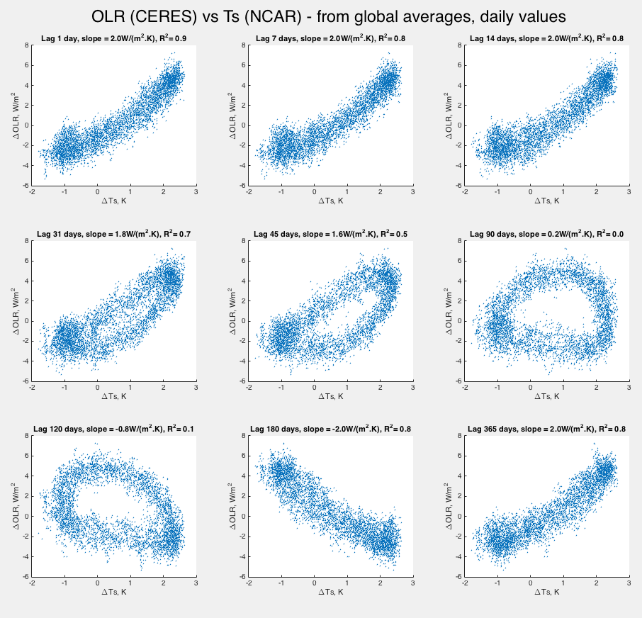
Figure 1 – Click to Expand
The slope gives the “apparent feedback” and the R² simply reflects how much of the graph is explained by the linear trend. This last value is easily estimated just by looking at each graph.
For reference, here is the timeseries data, as anomalies, with the temperature anomaly multiplied by a factor of 3 so its magnitude is similar to the OLR anomaly:
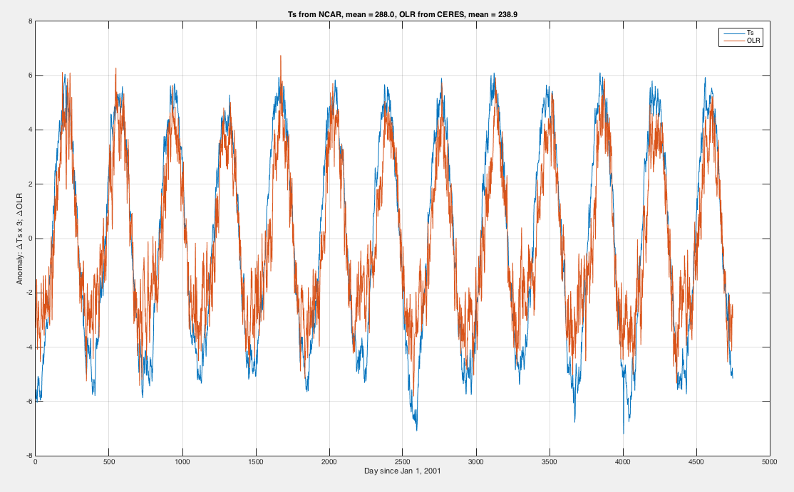
Figure 2 – Click to Expand
Note on the calculation – I used the daily data to calculate a global mean value (area-weighted) and calculated one mean value over the whole time period then subtracted it from every daily data value to obtain an anomaly for each day. Obviously we would get the same slope and R² without using anomaly data (just a different intercept on the axes).
For reference, mean OLR = 238.9 W/m², mean Ts = 288.0 K.
My first question – before even producing the graphs – was whether a lag graph shows the change in OLR due to a change in Ts or due to a mixture of many effects. That is, what is the interpretation of the graphs?
The second question – what is the “right lag” to use? We don’t expect an instant response when we are looking for feedbacks:
- The OLR through the window region will of course respond instantly to surface temperature change
- The OLR as a result of changing humidity will depend upon how long it takes for more evaporated surface water to move into the mid- to upper-troposphere
- The OLR as a result of changing atmospheric temperature, in turn caused by changing surface temperature, will depend upon the mixture of convection and radiative cooling
To say we know the right answer in advance pre-supposes that we fully understand atmospheric dynamics. This is the question we are asking, so we can’t pre-suppose anything. But at least we can suggest that something in the realm of a few days to a few months is the most likely candidate for a reasonable lag.
But the idea that there is one constant feedback and one constant lag is an idea that might well be fatally flawed, despite being seductively simple. (A little more on that in note 3).
And that is one of the problems of this topic. Non-linear dynamics means non-linear results – a subject I find hard to describe in simple words. But let’s say – changes in OLR from changes in surface temperature might be “spread over” multiple time scales and be different at different times. (I have half-written an article trying to explain this idea in words, hopefully more on that sometime soon).
But for the purpose of this article I only wanted to present the simple results – for discussion and for more analysis to follow in subsequent articles.
Articles in the Series
Part One – introducing some ideas from Ramanathan from ERBE 1985 – 1989 results
Part One – Responses – answering some questions about Part One
Part Two – some introductory ideas about water vapor including measurements
Part Three – effects of water vapor at different heights (non-linearity issues), problems of the 3d motion of air in the water vapor problem and some calculations over a few decades
Part Four – discussion and results of a paper by Dessler et al using the latest AIRS and CERES data to calculate current atmospheric and water vapor feedback vs height and surface temperature
Part Five – Back of the envelope calcs from Pierrehumbert – focusing on a 1995 paper by Pierrehumbert to show some basics about circulation within the tropics and how the drier subsiding regions of the circulation contribute to cooling the tropics
Part Six – Nonlinearity and Dry Atmospheres – demonstrating that different distributions of water vapor yet with the same mean can result in different radiation to space, and how this is important for drier regions like the sub-tropics
Part Seven – Upper Tropospheric Models & Measurement – recent measurements from AIRS showing upper tropospheric water vapor increases with surface temperature
Part Eight – Clear Sky Comparison of Models with ERBE and CERES – a paper from Chung et al (2010) showing clear sky OLR vs temperature vs models for a number of cases
Part Nine – Data I – Ts vs OLR – data from CERES on OLR compared with surface temperature from NCAR – and what we determine
Part Ten – Data II – Ts vs OLR – more on the data
References
Wielicki, B. A., B. R. Barkstrom, E. F. Harrison, R. B. Lee III, G. L. Smith, and J. E. Cooper, 1996: Clouds and the Earth’s Radiant Energy System (CERES): An Earth Observing System Experiment, Bull. Amer. Meteor. Soc., 77, 853-868 – free paper
Kalnay et al.,The NCEP/NCAR 40-year reanalysis project, Bull. Amer. Meteor. Soc., 77, 437-470, 1996 – free paper
NCEP Reanalysis data provided by the NOAA/OAR/ESRL PSD, Boulder, Colorado, USA, from their Web site at http://www.esrl.noaa.gov/psd/
Notes
Note 1: Boring Detail about Extracting Data
On the plus side, unlike many science journals, the data is freely available. Credit to the organizations that manage this data for their efforts in this regard, which includes visualization software and various ways of extracting data from their sites. However, you can still expect to spend a lot of time figuring out what files you want, where they are, downloading them, and then extracting the data from them. (Many traps for the unwary).
NCAR – data in .nc files, each parameter as a daily value (or 4x daily) in a separate annual .nc file on an (approx) 2.5º x 2.5º grid (actually T62 gaussian grid).
Data via ftp – ftp.cdc.noaa.gov. See http://www.esrl.noaa.gov/psd/data/gridded/data.ncep.reanalysis.surface.html.
You get lat, long, and time in the file as well as the parameter. Care needed to navigate to the right folder because the filenames are the same for the 4x daily and the daily data.
NCAR are using latest version .nc files (which Matlab circa 2010 would not open, I had to update to the latest version – many hours wasted trying to work out the reason for failure).
CERES – data in .nc files, you select the data you want and the time period but it has to be a less than 2G file and you get a file to download. I downloaded daily OLR data for each annual period. Data in a 1ºx 1º grid. CERES are using older version .nc so there should be no problem opening.
Data from http://ceres-tool.larc.nasa.gov/ord-tool/srbavg
AIRS – data in .hdf files, in daily, 8-day average, or monthly average. The data is “ascending” = daytime, “descending” = nighttime plus some other products. Daily data doesn’t give global coverage (some gaps). 8-day average does but there are some missing values due to quality issues. Data in a 1ºx 1º grid. I used v6 data.
Data access page – http://disc.sci.gsfc.nasa.gov/datacollection/AIRX3STD_V006.html?AIRX3STD&#tabs-1.
Data via ftp.
HDF is not trivial to open up. The AIRS team have helpfully provided a Matlab tool to extract data which helped me. I think I still spent many hours figuring out how to extract what I needed.
Files Sizes – it’s a lot of data:
NCAR files that I downloaded (skin temperature) are only 12MB per annual file.
CERES files with only 2 parameters are 190MB per annual file.
AIRS files as 8-day averages (or daily data) are 400MB per file.
Also the grid for each is different. Lat from S-pole to N-pole in CERES, the reverse for AIRS and NCAR. Long from 0.5º to 359.5º in CERES but -179.5 to 179.5 in AIRS. (Note for any Matlab people, it won’t regrid, say using interp2, unless the grid runs from lowest number to highest number).
Note 2: Checking data – because I plan on using the daily 1ºx1º grid data from CERES and NCAR, I used it to create the daily global averages. As a check I downloaded the global monthly averages from CERES and compared. There is a discrepancy, which averages at 0.1 W/m².
Here is the difference by month:
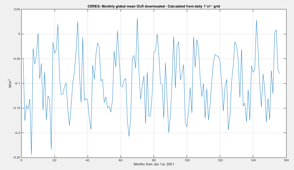
Figure 3 – Click to expand
And a scatter plot by month of year, showing some systematic bias:
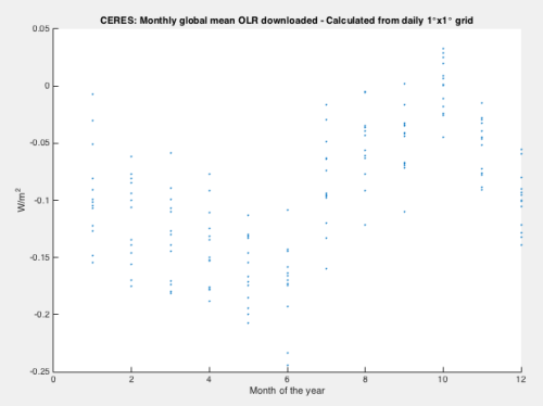
Figure 4
As yet, I haven’t dug any deeper to find if this is documented – for example, is there a correction applied to the daily data product in monthly means? is there an issue with the daily data? or, more likely, have I %&^ed up somewhere?
Note 3: Extract from Measuring Climate Sensitivity – Part One:
Linear Feedback Relationship?
One of the biggest problems with the idea of climate sensitivity, λ, is the idea that it exists as a constant value.
From Cloud Feedbacks in the Climate System: A Critical Review, Stephens, Journal of Climate (2005):
The relationship between global-mean radiative forcing and global-mean climate response (temperature) is of intrinsic interest in its own right. A number of recent studies, for example, discuss some of the broad limitations of (1) and describe procedures for using it to estimate Q from GCM experiments (Hansen et al. 1997; Joshi et al. 2003; Gregory et al. 2004) and even procedures for estimating from observations (Gregory et al. 2002).
While we cannot necessarily dismiss the value of (1) and related interpretation out of hand, the global response, as will become apparent in section 9, is the accumulated result of complex regional responses that appear to be controlled by more local-scale processes that vary in space and time.
If we are to assume gross time–space averages to represent the effects of these processes, then the assumptions inherent to (1) certainly require a much more careful level of justification than has been given. At this time it is unclear as to the specific value of a global-mean sensitivity as a measure of feedback other than providing a compact and convenient measure of model-to-model differences to a fixed climate forcing (e.g., Fig. 1).
[Emphasis added and where the reference to “(1)” is to the linear relationship between global temperature and global radiation].
If, for example, λ is actually a function of location, season & phase of ENSO.. then clearly measuring overall climate response is a more difficult challenge.


SOD: There may be some confusion about the meaning of temperature anomaly in this post. I presume that the 3.5 degC range in these plots is the seasonal change in mean global surface temperature due to the lower surface heat capacity in the northern hemisphere. When assessing CLIMATE change, seasonal changes are often removed by converting data to temperature “anomalies” by subtracting the average monthly temperature for a reference period from each month’s reading. This method of producing anomalies removes all seasonal signals from the data.
(Assuming I understand what you have done) when looking at the graphs in Figure 1 with little lag, the data on the left are coming from the planet when it is summer in the southern hemisphere and winter in the northern hemisphere. The data on the right are coming from the planet when it is summer in the northern hemisphere and winter in the southern hemisphere. So you are analyzing SEASONAL differences in OLR averaged over the whole planet – with large differences in ocean coverage between the two hemispheres. This makes me wonder what happens in smaller regions that might be more homogeneous – for example 30-40 degN over the ocean. Global feedback is the sum of many such regional feedbacks.
Frank,
You are correct I did not create monthly anomalies.
One of my initial thoughts was that removing the monthly average or the seasonal average (DJF, MAM, JJA, SON) and looking at the slope may introduce some kind of artifact.
Next up I will remove the monthly average and then the seasonal average and we will see how this affects the result.
Likewise we can look at regions.
You didn’t do anything wrong – you simply used the term anomaly in a context that might be misunderstood by people who focus on data from individual stations or the global surface temperature anomaly reported by GISS, BEST, Hadley, etc. Taking anomalies would have eliminated all of the useful seasonal signal (which many people don’t realize is roughly the same size as “future global warming”).
I’d love to see regional information. I’ve looked for information on how well climate models reproduce regional seasonal changes and not found much information. AR4 had some information, but it was presented in a format that was hard to interpret – seasonal variability reported as standard deviation.
SOD: In Figure 2, you multiplied the temperature anomaly by 3 before plotting. If you take the derivative of the S-B equation and do a little algebra, you can derive – for a blackbody or graybody with no feedback:
dW/W = 4*(dT/T)
If you had chosen a factor of 4 (rather than 3), the amplitude of the observed OLR curve would be about 70% of that expected for clear skies with no feedback.
I didn’t explain this properly. If you express the change in radiation and temperature as a fraction or percentage (dW/W and dT/T), they are related by the above equation. A 1% change in surface temperature (2.9 degK) produces a 4% change in radiation (9.6 W/m2) from a simple blackbody OR gray body (without feedbacks). The seasonal cycle in GMST is about 3.5 degK (1.2% change) and – without feedbacks – would be associated with a 4.8% change in OLR (11.6 W/m2).
The amplitude of the seasonal change in OLR is only about 8 W/m2 in Figure 2, because water vapor absorbs some of the increased surface OLR and negative lapse rate feedback (more warming in the troposphere than at the surface) negates about half of this effect.
[ moderator’s note – deleted due to relevance, or lack thereof]
[emphasis added]
I believe you mean more rather than less.
Thanks – I fixed the article.
SoD,
I note there is a very wide range in the global Ts. I presume that is due to the fact that the global average temperature swings by about 3-4C every 6 months due to perihelion/aphelion and hemispheric asymmetry. Maybe I’m wrong, but wouldn’t that taint or skew the relationship you’re trying to determine?
RW,
I think the seasonal cycle is the reason why we see the relationships move once we get to 90 days lag and reverse once we are at 180 days lag.
RW wrote: “I note there is a very wide range in the global Ts. I presume that is due to the fact that the global average temperature swings by about 3-4C every 6 months due to perihelion/aphelion and hemispheric asymmetry. Maybe I’m wrong, but wouldn’t that taint or skew the relationship you’re trying to determine?
The relationship will be skewed to some extent. By studying the seasonal cycle in temperature and OLR from clear skies, we are trying to learn about how OLR from clear skies will change as the globe warms. Seasonal change involves a large warming in the NH – perhaps averaging 7.5 degC (12 degC over land and 5 degC over ocean) – and a smaller cooling in the SH – perhaps averaging -4 degC (-3.0 degC over ocean and -8.0 degC over land). These number are illustrative GUESSES that produce a net seasonal change of 3.5 degC, given fact that NH is 40% land and the SH is 20% land. If climate sensitivity for 2XCO2 were 3.5 degC, both hemispheres would eventually warm about this amount (but possibly not equally). In both seasonal and global warming, the warming at high latitudes is bigger than the warming at low latitudes. To the extent that water vapor plus lapse rate feedback is linear within this range, hemispheric asymmetry shouldn’t matter. For example, the 7%/degC increase in saturated water vapor pressure is fairly linear. Moist and dry adiabatic lapse rate are fairly linear with temperature, but the fraction the troposphere where the lapse rate determined by adiabatic considerations differs from hemisphere to hemisphere and presumably season to season.
http://www.srh.noaa.gov/jetstream/upperair/skewt.htm
Other relationships are skewed or worse. Satellites monitor the seasonal cycle in SWR reflected from clear skies – i.e. surface albedo. Since seasonal snow cover is much greater in the NH than the SH, the seasonal cycle in reflected SWR from clear skies has nothing to do with the amount of ice-albedo feedback that will accompany global warming. The SH has more cloud cover than the NH, so deducing “global” cloud feedback from the seasonal changes in OLR and reflected SWR is also problematic.
FWIW, climate models do a good job of predicting the observed seasonal cycle in OLR from clear skies. Either the models get the increase in humidity with temperature about right, or there are compensating errors in humidity and lapse rate. (It is possible that this agreement exists because some model parameters have been tuned so that the seasonal change in OLR from clear skies is about 8 W/m2.) The models do a lousy – and mutually inconsistent – job with the seasonal cycle in reflected SWR from clear and cloudy skies and OLR from cloudy skies.
On second thoughts, the relationship we are seeing – as Frank explains – is the seasonal cycle response.
And that is why when the lag goes to 180 days we see the opposite slope.
So the “OLR response” to the change in temperature imposed by the perihelion/aphelion and hemispheric land asymmetry is apparently a positive feedback.
More in upcoming graphs..
Ocean heat transport also shows seasonal changes. Ocean heat transport models indicate changes in ocean heat transport causes dynamical changes in water vapor above that expected from just a change in temperature and that this dynamical change in water vapor causes warming. It is one of the ways ocean heat transport is hypothesised to cause warming. Chicken or egg?
In fact the graphs resemble classic Lissajous patterns you get when you apply oscillations of the same frequency but out of phase to the x and y axis of an oscilloscope – which is more or less what you are doing.
I agree with DeWitt Payne.
SOD,
I have looked at something similar which I have posed here for the seasonal, not shorter term variation.
By calculating the “emissive temperature” from the OLR and plotting it versus the surface temperature, the depiction of the greenhouse effect and of feedback become apparent:
SoD,
Very interesting. As you recognize, a key issue is whether the slope is the thing you would like it to be (feedback parameter), or something related to it in a possibly complicated way. Something I really liked in the Chung et al. paper is that they tested that by applying their analysis to models for which the feedback is known. I think that would be interesting to try here.
If a model gives graphs similar to observations for the various lags, it would imply that the model is getting something important right. If it gives very different results, then the model is significantly wrong. If the slopes for the graphs for various models vary in a systematic way with feedback strength, then the model that is closest to the observations might well be the one with the most suitable feedback.
Mike M and SOD: The average water molecule remains in the atmosphere for something like 9 days (total precipitable water column divide by average precipitation per day). The atmosphere and surface continuously exchange several hundred W/m2 of DLR and OLR. The time scale for convection is a little harder to assess. Thunderstorms seem to boil up and disperse in a day, or at least move hundreds of miles per day. Convection and precipitation associated with weather fronts behaves similarly. In the tropics, the Madden Julian oscillation moves areas of deep convection east about 200-400 day. I can’t think of anything that would justify a lag between Ts and OLR of more than about a week.
On the other hand, Roy Spenser says:
“It should be remembered that during ENSO, there is a 1-2 month lag between sea surface temperature change and tropospheric temperature changes, so the tropospheric temperature anomaly will take a month or two to reflect what recent global SSTs have been doing. that it takes 1-2 months for the heat in elevated SST during El Nino to be transferred to the upper troposphere”
http://www.drroyspencer.com/2014/11/uah-global-temperature-update-for-october-2014-0-37-deg-c/
Double-checking on Roy’s information produced the following reference and a larger set of complications that torpedoed my simple-minded thought. When a Kelvin wave delivers heat to the surface, the troposphere responds in 1 to 2 weeks. On the other hand, the troposphere warming lags SST warming by 3-6 tmonths during the usual evolution of El Nino. It seems there is a two-way interaction between SSTs and the troposphere and the depth of the mixed layer is important to the lag. El Nino produces lagged SST anomalies outside the Equatorial Pacific via the atmosphere
http://journals.ametsoc.org/doi/full/10.1175/JCLI3514.1
So, if you look at regions, you may find different lagged relationships than you found for the globe as a whole.
Frank,
You wrote ” The average water molecule remains in the atmosphere for something like 9 days (total precipitable water column divide by average precipitation per day). The atmosphere and surface continuously exchange several hundred W/m2 of DLR and OLR”.
But most water vapor is in the boundary layer and most of the exchange is in and out of the boundary layer. The lifetime of water vapor in the mid to upper troposphere, which is where the greenhouse effect happens, is likely longer.
Global average water vapour correlates well with global average temperature at the monthly timescale:

Mike M wrote: “But most water vapor is in the boundary layer and most of the exchange is in and out of the boundary layer. The lifetime of water vapor in the mid to upper troposphere, which is where the greenhouse effect happens, is likely longer.”
You raise a good point. However, I’m under the impression that precipitation falls mostly after water vapor has risen above the boundary, the the lifetime of water vapor at altitudes capable of exerting a strong GHE could be the same as for the atmosphere as a whole. Nevertheless, the lifetime of water vapor in slowly descending regions or stagnant regions like the stratosphere might be very different and forcing is presumably proportional to the log of the concentration.
If I wasn’t clear above, I found that my simple-minded idea that fast feedbacks happen within days was wrong during the development of an El Nino. The introduction to the paper I linked had many references to lags between surface and troposphere.
TE,
Could you convert that chart to relative humidity rather than TPW. A linear correlation of temperature to TPW would imply that RH isn’t constant, as saturation water vapor pressure is an approximately exponential function of temperature. Of course it’s possible that the temperature swing isn’t large enough for the non-linearity to make a difference. I’d do it myself if you had put in links to the data. If RH decreases with temperature, then the positive feedback from water vapor is smaller.
Ya – the data,
http://nomads.ncdc.noaa.gov/data/cfsrmon/197901/
are a ton of monthly grib files, so I used PW as a single measure, even though PW is for the entire depth of atmosphere, not just the surface.
It does invoke the question of the profile of water vapor feedback – if water
vapour increased in absolute terms, but only in the boundary layer, the effect would be different than if water vapour increased aloft, but not at the surface.
The relative humidity aloft in the sub-tropics is very low. Notional diagrams depict de-training from the ITCZ moistening the sub-tropics to maintain constant RH, but I wonder how uniform an increase in RH really is. Some regions of the atmosphere are close to zero RH than they are to the C-C limit.
Oh yeah, should remember that the earth’s temperature and these correlations are dominated by the NH because of land mass. The same patterns occur in the SH, just of a smaller extent:

I could use MODTRAN data to see how TPW changes with temperature at constant RH. MODTRAN only varies the data below 13km when changing surface temperature. There is substantial curvature of the saturated absolute humidity vs temperature from 280-300K. The exponential fit to the data is 4E-07*exp(0.601*T)
Click to access Blanchette2015.pdf
This paper shares a lot of the vocabulary of this SOD article, and has some interesting result on OLR, tropospheric humidity and surface temperature by looking at OLR spectrum. I have no idea how it fits with what you are doing here but I hope its useful. Do you know of any other work where the OLR is analysed to understand the evolution of various forcings and feedbacks? It seems like a interesting approach.
“Do you know of any other work where the OLR is analysed to understand the evolution of various forcings and feedbacks? It seems like a interesting approach.”
I think pretty much the entire field looks at how OLR changes with temperature to diagnose and quantify feedback.
of course you’re right RW, I stupidly left out the most important word in that question – spectrum.
Teh question should have been
Do you know of any other work where the OLR SPECTRUM is analysed to understand the evolution of various forcings and feedbacks?
human1ty1st: I found this paper fascinating. Observation from space usually involve total OLR or measurements of individual components of the system – usually in the microwave region, not IR: troposphere temperature (UAH and RSS), sea surface temperature and wave vapor. So it was interesting to see the change in OLR vs wave length over a decade – and somewhat disconcerting:
1) Emission through the atmospheric window is down because surface temperature is lower due to the hiatus (which now allegedly isn’t real)?
2) Emission from the CO2 band is lower because increasing CO2 is raising the characteristic emission level? If lower surface temperature is reducing OLR through the atmospheric window, why can’t reduced emission from the CO2 band be evidence of lower temperature in the upper atmosphere?
3) Increased emission from water vapor bands is caused by lower temperature and constant relative humidity?
If one looks at the Schwarzschild equation for the change in OLR (dI) at a given wavelength as it passes through an increment of distance (ds):
dI/ds = n*o*B(lamba,T) – n*o*I_0
you see that the change is a complicated function of n (GHG concentration), T (local temperature) and I_0 (incoming OLR). I’m skeptical that the authors can definitively assign the change at any particular wavelength to any particular cause without a more careful analysis. Doing the job right, however, would be a large undertaking.
The AIRS team abstracts about a dozen parameters for individual grid cells (temperature, water vapor, CO2, ozone, etc) from the spectrum, but the process must involve fitting a complicated model to the spectral data.
http://airs.jpl.nasa.gov/data/physical_retrievals
This paper lets one see the overall change in the OLR spectrum from space – but IMO can’t convincingly assign causes. Elsewhere we get information about individual causes (SST and SAT, UAH/RSS, CO2, humidity), but usually see only their aggregate impact on OLR.
Frank,
The shape of the trend curve for the wing of the CO2 band between 650 and 800 cm-1 is consistent with a change in CO2 concentration, not a change in temperature. Besides, the temperature hasn’t changed very much.
DeWitt wrote: “The shape of the trend curve for the wing of the CO2 band between 650 and 800 cm-1 is consistent with a change in CO2 concentration, not a change in temperature. Besides, the temperature hasn’t changed very much.”
Thanks for the reply.
The “temperature hasn’t changed very much” at what altitude? RSS, UAH and others offer a suite of temperature “products”. Which one is appropriate for the “wing of the CO2 band”? The author of the paper cite the hiatus in warming, but they don’t specify which temperature record.
I may be missing something, but it isn’t obvious why the shape of the trend curve between 650 and 800 cm-1 is appropriate for a change in CO2 concentration rather than a change in temperature. In the emission term of the Schwarzschild eqn, n*o*B(lamba,T), I’m sure you can’t tell the difference between a change in n and a change in T. However, we do need to account for both emission and absorption:
dI/ds = n*o*[B(lamba,T) – I_0]
The behavior of the term in [brackets] isn’t obvious to me since, I_0 also depends on T (and n and o) lower in the atmosphere.
I plotted the difference in MODTRAN spectra for 476 and 496 ppmv CO2 (2003 and 2013 average) and for a change in surface temperature of 1K, which also changes the temperature profile up to 13km, at constant CO2. The CO2 difference curve is a negative peak that returns to about the same baseline at 800 cm-1 like the graph in the paper. The temperature curve, OTOH, is a decline to a lower level, as would be expected because that wing of the CO2 band borders on the window region.
Needless to say, the temperature didn’t change by anywhere close to 1K from 2003 to 2013. It’s more like 0.1K. A change of 0.1K would be very close to zero difference.
Thanks DeWitt. If I understand correctly, the fingerprint for a temperature shift is a change in the atmospheric window and we assume a constant lapse rate to estimate what happens at other wavelengths. Changes caused by an increase in CO2 are localized in the CO2 band, but can be complicated once altitudes are involved where the lapse rate is zero or negative. (I presume you chose the US Standard Atmosphere.)
1976 US Standard Atmosphere, although I suspect that the pattern would be similar with other atmospheres. OLR through the window would depend strongly on surface temperature and weakly on other factors. For a small change in temperature, I think a constant lapse rate is a safe assumption.
human1ty1st,
Thanks for the link to the Blanchette paper. It is an interesting approach, but I am skeptical as to the value of the results. The changes in emission at any given wavelength will be *very* small, so extremely careful attention to possible errors is required to get a useful result. You have to worry about random noise in the data, drift in the instruments, and how changes in cloudiness (or even the spatial distribution of clouds) might affect brightness temperature. They do not seem to have done any of that.
And the results don’t seem to make sense. An instantaneous doubling of CO2 would produce a change in brightness T of 1.1 K which would then decrease with time. So the change in one decade should be *much* less than 1.1 K. But they get about half that, and they let it pass without comment. My guess is that all the “results” are artifacts of the analysis procedure.
I just noticed that this is published in the “McGill Science Undergraduate Research Journal”. So it is some student’s summer project or senior project. By that standard, it is OK.
Thanks for the reference to the Blanchette paper. Can anyone explain the magnitude of the temperature trends which appear in Figure 2a?
Are we to understand that this level of decadal temperature decrease has been used to balance the books?
SoD –
I welcome your interest in these datasets, as I’m sure there’s information there, and naive interpretation by others will only add to the muddle.
You may be a victim of the ambiguous language in general use in climate science. For some clarification I offer the following:
Water-vapour moves in our atmosphere largely by passive transport in moving air. The atmosphere is closed, so large-scale movement is part of a circulation or loop. In a closed loop, cause and effect become ambiguous. Also, you cannot understand a loop from only a part of it. You may have an open-loop model, with well-defined “in” and “out” linked by a causal chain with “gain” elements etc but are forbidden feedbacks; or a loop model with arbitrary “in” and “out” linked by a transfer-function, all the feedbacks you wish, but no causation. I think what you’re attempting is the latter.
A CERES map of clear-air OLR at an equinox shows a notable large-scale uniformity, particularly in the tropics. This suggests (to me) that most of that OLR is from high air, which by circulation won’t correlate with the surface below (except on the “loop” scale). As the Hadley cell has a characteristic time of weeks, you might find a transient correlation close to the ITCZ (“in-loop”), but need much longer to estimate the loop response (by which time the season’s changed…).
BTW exceptions to the tropical OLR uniformity appear to be where the lower half of the atmosphere is replaced by mountain, and where the surface is jungle. If your aim is a “typical-Earth” estimate, you might consider excluding those areas (and perhaps India/Tibet).
I remember using scatter diagrams for process control in my engineering career. A pattern with a hole in it signaled that an unknown control variable existed.
SoD,
Interesting. Interpretation of these results is problematic for a number of reasons. If you consider a model where the Earth is subdivided into n latitude zones, then the global (seasonal) temperature variation which you are tracking here can be approximated as the resolved summation of n annual temperature oscillations, one for each latitude zone, each of different amplitude and with adjacent zones slightly out of phase with each other. All else being equal, this means that at best a crossplot of aggregate OLR against average temperature change is telling you something about the system response to a change in the weighting of the latitudinal feedbacks. It is not obvious that the OLR gradient can yield any useful information about the system response to a general warming, which is perhaps the more pertinent question. (Think of the aggregate OLR response as the scalar product of two n-dimensional vectors in feedback and deltaT, and consider what perturbations you are actually testing here.)
However, all else is not equal in this instance. During the annual cycle, there is a lot more going on that a simple change in how forcing from solar insolation is distributed around the planet. There is a well-documented annual and semiannual cycle apparent in Length of Day. Energy, in the form of a momentum flux, is added to and subtracted from the Earth via its change in axial angular velocity. This has a direct effect on Atmospheric Angular Momentum, and importantly for your analysis, on the meridonial flux and the vertical temperature profile of mid- and upper- atmosphere. The only point I would make here is that this is an orbitally driven phenomenon, and not a temperature-driven phenomenon, and one which changes the local feedback if expressed as the local gradient of OLR vs surface temperature change. It is not obvious to me why we should assume that its effects, via internal redistribution of heat, on the relationship between aggregate OLR and average surface temperature should be similar to the effect of a model-predicted change (i.e. increase) in meridonial flux arising from a general warming.
All in all, I believe that a simple interpretation of feedbacks from the seasonal cycle may just not be possible.
Hi Paul K,
Do you know, or have a reference to the magnitude of energy flux due to seasonal change in rotational velocity? My impression was that this is a very small factor.
WRT the complexity of relating the seasonal cycle in global temperature to OLR: I completely agree that there is probably too much going on to gather much reliable information on climate sensitivity from the seasonal variations in global average temperature and measured OLR. But I do find it interesting that the curvature of OLR vs temp anomaly (first row, figure 1) at least hints the sensitivity is lower (steeper slope) at higher temperature. Strong positive feedbacks would likely give less slope (greater sensitivity) at higher temperature. I also find it interesting that the average slope (~2 watts/M^2/degree) is not far from the slope you would expect if climate sensitivity is near the value Nic Lewis estimates from long term energy balance estimates…. 3.71/2 = 1.85 degrees per doubling of CO2.
Hi Steve,
I have not seen a full calculation of annual energy exchange attempted anywhere. No doubt the net gain for the atmosphere alone could be calculated using the same information that goes into the observations for AAM, but I have not seen it done.
Calculation from first principles is difficult. We can easily estimate the change in rotational energy of the solid body of the Earth. The average annual change in LOD is around 3ms from peak to trough. Using a moment of inertia of 7.04E37 kg.m^2 for the Earth, the change in rotational kinetic energy works out to be about 1.3E22 joules – gained and lost each year.
This is not a negligible quantity. However, we cannot assume that this loss (gain) of solid body rotational energy is matched by a corresponding gain (loss) of energy to the hydrosphere and the atmosphere. Some of the energy exchange is known to be with the moon via a gravitational torque. So the energy of the total Earth system is not conserved. On the other hand, we can assume to a good first order approximation that total angular momentum of the Earth system is conserved. This explains the almost perfect correlation between LOD and AAM for high frequency (<10 years) variation.
More importantly, perhaps I misled you with my first comment. I did not mean to suggest that SoD's estimate of greenhouse effect is suspect because of the magnitude of energy gain/loss by the climate system; this would be more of a problem if SoD were attempting an energy balance, but he is not. What I was suggesting is that the feedback calculation is suspect because of the nature of the changes. During the annual cycle, the atmospheric circulation changes substantially because of (a) non-uniform heating and (b) net energy gain/loss from a momentum flux. (This latter is reflected in the oscillation of AAM, as we would expect.) This results in a redistribution of winds, clouds and sensible heat flux during the annual cycle which is recurrent and predictable, at least in very broad terms. So at the local level, a change in OLR is reflecting both an oscillatory change in local temperature AND an oscillatory change in net heat flux in or out of that locale. At the global level, the change in aggregate OLR is reflecting a change in the spatial weighting of the outgoing flux, and, similarly, the change in average temperature is reflecting a change in the spatial distribution of temperature around the globe . It seems to me difficult to defend an assumption that this relationship should be similar to the change in aggregate OLR which we would expect from a more uniform warming over decades to centuries. In the latter case, we can assume that the “average atmospheric circulation” stays unchanged from year to year, apart from some anticipated secular increase in meridonial flux.
I agree with you about the coincidence of feedback values. So it could be that my fears about unsafe assumptions are unjustified. On the other hand, it is possible that both estimates are inaccurate. It seems dangerous to use an unsafe estimate as a calibration point to support another slightly less unsafe estimate.
Paul,
Thanks for your comment. The calculated energy from change in LOD is a lot higher than I would have guessed. But my doubt is how much of that is really an energy change, and how much might be due to a change in the angular inertia of the Earth. I mean, seasonal relocation of mass from low latitude with high tangential velocity to high latitude (with low tangential velocity) and back, as we might expect due to a seasonal build of land supported snow and ice in the northern hemisphere, followed by summertime melt, would cause the Earths rotation to speed and slow slightly with the mass distribution. I will plug in some plausible numbers for mass redistribution and see how much change in LOD might be expected. What time of year has the shortest and longest LOD?
Hi again Paul,
I did a little digging; the minimum length of day is in February of each year (with some short term variation superimposed on the seasonal trend). Here is the interesting thing for me: the seasonal sea level variation almost exactly matches the seasonal variation in LOD, with lowest sea level in February of each year, as you would expect for seasonal redistribution of water mass as snow/ice at high northern latitudes. Could be coincidence, of course. I will try to plug in some plausible numbers and estimate a LOD effect.
Steve,
This thesis of Simon Driscoll may answer the main questions.
The page 22 explains:
Those are the most important points as far as I understand. Atmospheric effects dominate on seasonal and shorter term, and jet streams are the most important component of the atmosphere. Further details and comparisons with empirical data can be found from the thesis.
When angular momentum is conserved, total rotational energy is not, but that’s not a problem as free energy from the solar heating of the surface can easily provide the energy needed, when rotational energy increases and dissipation to thermal energy do the opposite.
Paul_K: A simple interpretation of feedbacks from the seasonal cycle is difficult. A comparison between the observed and modeled seasonal cycle clearly exposes inadequacies in climate models because the change is large (3.5 degK) and can be monitored 10 times per decade. The difference between observed and modeled climate change over a decade is much smaller and can be observed only once.
franktoo:
I agree. Demonstrating that a finely-gridded fully implicit GCM can match the (local) amplitudes of variation in temperature, TOA fluxes and atmospheric circulation over a couple of cycles of the QBO would go some way towards answering the question of whether there are any key pieces missing or incorrectly characterised. Upscaling from such a model to a coarser system would then have rather more credibility than the present suite of models.
Paul_K: What I find very surprising is that models produce very different responses to the 3.5 degK increase in GMST that takes place every year (the “seasonal cycle” that disappears when temperature anomalies are calculated). All models produce the same annual increase in OLR from clear skies similar to that observed from space, perhaps because they have been tuned to do so. (That means they get WV+LR lapse rate feedback about right on a global scale.) Climate models disagree with each other and with observations from space about seasonal changes in OLR from cloudy skies, SWR from cloudy skies and SWR from clear skies. (Changes in SWR from clear skies are driven by seasonal changes in snow cover, somewhat related to ice-albedo feedback.)
Click to access 7568.full.pdf
Paul K,
I agree.
I’ve made many similar statements in various past articles.
Off topic – there is some discussion on About this Blog on ocean chemistry. I don’t know anything about ocean chemistry except there is some salt in there.
Comments on blog pages appear in the “Recent Comments” section, but comments on the fixed pages (Etiquette, About..) don’t appear there for some reason.
[…] « Clouds & Water Vapor – Part Nine – Data I – Ts vs OLR […]
[…] Part Nine – Data I – Ts vs OLR we looked at the monthly surface temperature (“skin temperature”) from NCAR vs OLR […]
Dear SoD
I have got good answers to my questions before, so i try again.
I have not been able to find any estimates of the change in forcing (radiation balance at TOA) versus the change in water vapor content (% rh).
It is strange because it is said that any temperature change will change the humidity (7%/K) and this will amplify the original temperature change 2 to 3 times more. Is water vapor the only GHG that can change temperature without changes i radiation?.
A simple estimation gives me 0.4W/m2 / %rh, based on the radiation change needed to amplify the temperature.
Can you find any estimates?
Svend: CMIP5’s estimate for water vapor feedback is 1.6 +/- 0.3 W/m2/K. If you assume water vapor rises an average of 7% for every degK increase in GMST (the exact number differ with local Ts and altitude), you get 0.23 W/m2/%.
A more rigorous way to do this is to use radiative transfer calculations. The online Modtran package allows you to increase the “water vapor scale” factor from 1.00 to 1.07, increasing the amount of water vapor at all altitudes by 7% (in the same way it allows you to increase CO2 from 300 to 600 ppm. Unfortunately, this facility only calculates “local” changes in OLR using standard atmospheric soundings, not “global” changes in forcing (OLR at the TOA averaged over the entire planet). Some change in OLR for the above 7% increase (and in parenthesis for doubling CO2 300-600 ppm) are:
US standard atmosphere (no clouds): 1.0 W/m2. (3.0 W/m2)
Tropical atmosphere (no clouds): 1.6 W/m2. (3.3 W/m2)
Tropical atmosphere (altostratus clouds): 0.8 W/m2. (2.6 W/m2)
Clouds reduce the effect of any forcing agent, because they only influence OLR from cloud top to space, not the surface to space. Altostratus are the highest clouds, and were chosen here to illustrate the biggest possible influence. The lowest clouds have negligible impact. Myhre calculated the standard forcing for well-mixed GHGs by combining many such calculations for many scenarios around the planet, using the change in OLR at the tropopause (not the TOA). As you see, my crude emulation of his process is coming in a little low for CO2 and a little below 1.6 W/m2/7% estimate based on feedback.
If ECS were CMIP5’s mean of 3.3 K/doubling, then 2XCO2 would be associated with a 5.3 W/m2 reduction in OLR from increasing humidity acting as a GHG. If ECS were 1.8 (as suggested by EBMs), increasing water vapor would reduce OLR by 2.9 W/m2. In either case, it would be crudely correct to say water vapor feedback doubles warming effect of CO2.
Forcing is the temperature independent change in OLR produced by a GHG, while a feedback is the change in OLR caused BY a change in GMST. Since water vapor is changed BY temperature much faster than water vapor can increase temperature by acting as a GHG, climate scientist usually treat water vapor as a feedback and don’t publicize the radiative forcing it produces by acting as a GHG. As you can hopefully see from my discussion, the reduction in OLR water vapor causes by acting as a GHG is properly taken into account whether you consider it a forcing or a feedback. The latter is simpler, because you don’t need to make assumptions about ECS.
Many thanks for the answer even if i mixed my question up with rh and absolute content, You got it right.
I find it a bit funny, that no one wants to give a forcing figure for water vapor just because it is called a feedback?
Anyway my quick estimate was not way out, so i must have some basic understanding.
Svend wrote: “I find it a bit funny, that no one wants to give a forcing figure for water vapor just because it is called a feedback?”
Someone may have published a forcing for an increase in water vapor, but result would be pretty meaningless. After evaporation, the average water molecule remains in the atmosphere for 9 days. If you add it to a rising air mass (about half of the sky) which is saturated, it condenses immediately. You can’t “force” climate change with increasing water vapor. I like using Modtran to calculate a forcing for water vapor because it helps skeptic (including me) understand what happens when water vapor is treated as a feedback.
I often hear that the normal GHG’s can not do their job because water vapor anyway absorbs all.
I would like your comment to my own simple explanation:
In the lower atmosphere water wapor absorbs all in a short distance, but it does not matter what the absorber is, the gasses exchange vibration and energy and any of the gasses can radiate or absorb.
Higher in the atmosphere water vapor reduces and then the normal GHG’s do what they do.
It is complicated stuff, so i would like to know if my explanation has some merit.
Else i would like some still simple but better explanation.
Svend: You must remember that GHGs both absorb and emit thermal IR. The change in intensity of radiation, dI, of a particular wavelength, lambda, as it passes an incremental distance ds through an atmosphere is given by:
dI = -n*o*I*ds + n*o*[B(lambda,T)]*ds = n*o*[B(lambda,T) – I]*ds
where the first term is absorption (and is the differential form of Beer’s Law) and the second term is emission. n is the density of the GHG, o is the absorption cross-section for the GHG at the wavelength of interest, T is the local temperature, B(lambda,T) is Planck’s function, and I is the intensity of the radiation entering the ds increment. When the incoming radiation has an intensity I = B(lambda,T), dI = 0. Blackbody radiation exists where absorption equals emission (and Planck postulated such an equilibrium when he derives his law). The above is called Schwarzschild’s equation for radiation transfer, is discussed at SOD and Wikipedia, and is numerically integrated by Modtran. What the equation “says” is that absorption and emission combine to bring the intensity of radiation leaving any homogeneous material closer to “blackbody intensity” B(lambda,T) than the radiation entering it. If high intensity light enters, absorption dominates over emission and if low intensity light enters, emission dominates. The rate at which it approaches blackbody intensity is proportional to the density of absorbing/emitting GHGs and their absorption cross-section.
So, where the concentration of water vapor is high, radiation strongly absorbed by water vapor will have intensity appropriate for a blackbody at the local temperature. Every photon absorbed in these locations is replace by a newly emitted one. (IIRC, at the wavelength most strongly absorbed by CO2, 90% of the upwelling photons emitted by the surface have been absorbed within 1 m, AND replaced by the same number of new photons emitted by CO2.) Higher in the atmosphere, water vapor concentration is lower and it is colder. In that case, upwelling radiation emitted from below can have a higher intensity than locally emitted radiation, [B(lambda,T)], and there will be more absorption than emission and dI will be negative. Most radiative forcing in our atmosphere arises on the shoulders of strong absorptions, where a photon can travel a kilometer or so upward (colder) between emission and absorption. When you sum up all changes in dI from the surface to space, the average 390 W/m2 emitted by the surface has been reduced to 240 W/m2 at the edge of space. Going the other direction, DLR increases from 0 at the edge of space to 333 W/m2 at the surface.
Calculations (numerical integration) with multiple GHGs and a range of wavelengths are fundamentally the same, you just added up the emission and absorption caused by all of the absorbing/emitting species in the increment ds. You simply need an increment ds short enough that the intensity of the incoming radiation, I, can be treated as a constant over that range. As a practical matter, it is easier to integrate the net change, [B(lambda,T) – I] for each increment of ds, rather than the increments of absorption and emission, because the net change is effectively zero where n*o is large. So the ds increments can cover a few percent of the atmosphere at a time.
Svend,
I’ll give a conceptual model and then send you to the article that shows the details.
Conceptual
Consider the ocean – very high emissivity (that means it’s close to a “blackbody”, or perfect emitter of radiation) at typical ocean temperatures.
So it’s radiating according to σTocean4.
Now we add very high levels of water vapor at the top of the boundary layer above the ocean, let’s say 1km up. So the water vapor is close to a perfect emitter (not really true but this is a conceptual model).
So it’s absorbing all radiation from the ocean, and re-emitting radiation according to its temperature. So σT1km4.
T1km is about 6’C less than Tocean so the very high levels of water vapor have reduced emitted radiation from the surface.
If you take the highest amounts of water vapor to be at more like 500m above the surface then the temperature difference is 3’C.
Even supposing these cases, the question is really about where CO2 does most of its absorption and emission.
This actually depends very much on where in the CO2 band you look.
It turns out that the changes in CO2 that cause radiation balance changes are causing an effect from the surface right up to the top of the troposphere. Water vapor goes to something like 1/1000 its surface concentration at the top of the troposphere. And the water vapor effect is mostly a function of the square of the specific humidity. So if you go to 1/10 of the water vapor, you get 1/100 of the absorption/emission.
I’m over-simplifying. But if you follow this conceptual picture, yes water vapor can overwhelm CO2, but only very close to the surface which doesn’t really change the “greenhouse effect”.
Detail
These are fairly involved because atmospheric radiation in the presence of different concentrations of GHGs (e.g. CO2 and water vapor) at different heights is NOT intuitive.
I really recommend reading the whole series if you want to gain a better understanding.
But the key ones to answer this question:
Visualizing Atmospheric Radiation – Part Four – Water Vapor
Visualizing Atmospheric Radiation – Part Seven – CO2 increases
This series or articles inspired me a bit. I had one problem. No matter how hard I tried, a WV feedback of 1.8W/m2 was impossible to attain from radiative transfer models. Not even adapting a “radiative flux” approach, where upward (negative) flux and downward (positive) flux at the tropopause are just added up to attain the canonical 3.7W/m2 CO2 forcing, would help. Only here I realized radiative transfer models seem to get ignored on this question anyhow.
I on the other side ignored that OLC/Ts relation, cause it never made much sense to me. Now I paid a little more attention to it. The basic problem I was well aware of, is that the tropospheric temperature does not follow surface temperature over the course of the seasons. The annual temperature range (ATR) is a lot smaller on mountain tops than in the low lands. Also in high latitude winter we typically have inversions as a consequence.
Also while we have a global ATR of about 4K, that is because of the extensive land masses in the NH. In siberia the ATR can reach up to 60K, which has no counter part in the SH. So while global surface temperature varies by these 4K due to topography, it does not reflect a change in heat content of the surface/atmosphere system. That will rather go the opposite way, as we are closer to the sun in NH winter.
So we have a variable surface temperature and a relatively sluggish tropospheric temperature, and that is pretty unrelated to WV btw. Since most OLR comes from the troposphere, of course dOLR/dTs will NOT be as large as the “Planck Feedback”. Understanding this devation from theory as evidence of WV feedback would be an embarrassing blunder.
Do I get it right, that the whole idea of WV feedback in climate science is based on not understanding this very issue?
Do I get it right? In a word: no. I’d go into more detail, but you are so far off and I’m not bored enought to take the time. You clearly don’t understand the role of relative humidity in radiative transfer.