The Science of Doom

Water vapor trends is a big subject and so this article is not a comprehensive review – there are a few hundred papers on this subject. However, as most people outside of climate scientists have exposure to blogs where only a few papers have been highlighted, perhaps it will help to provide some additional perspective.

Think of it as an article that opens up some aspects of the subject.

And I recommend reading a few of the papers in the References section below. Most are linked to a free copy of the paper.

Mostly what we will look at in this article is “total precipitable water vapor” (TPW) also known as “column integrated water vapor (IWV)”.

What is this exactly? If we took a 1 m² area at the surface of the earth and then condensed the water vapor all the way up through the atmosphere, what height would it fill in a 1 m² tub?

The average depth (in this tub) from all around the world would be about 2.5 cm. Near the equator the amount would be 5cm and near the poles it would be 0.5 cm.

Averaged globally, about half of this is between sea level and 850 mbar (around 1.5 km above sea level), and only about 5% is above 500 mbar (around 5-6 km above sea level).

Where Does the Data Come From?

How do we find IVW (integrated water vapor)?

• Radiosondes
• Satellites

Frequent radiosonde launches were started after the Second World War – prior to that knowledge of water vapor profiles through the atmosphere is very limited.

Satellite studies of water vapor did not start until the late 1970’s.

Unfortunately for climate studies, radiosondes were designed for weather forecasting and so long term trends were not a factor in the overall system design.

Radiosondes were mostly launched over land and are predominantly from the northern hemisphere.

Given that water vapor response to climate is believed to be mostly from the ocean (the source of water vapor), not having significant measurements over the ocean until satellites in the late 1970’s is a major problem.

There is one more answer that could be added to the above list:

• Reanalyses

As most people might suspect from the name, a reanalysis isn’t a data source. We will take a look at them a little later.

Quick List

Pros and Cons in brief:

Radiosonde Pluses:

• Long history
• Good vertical resolution
• Can measure below clouds

Radiosonde Minuses:

• Geographically concentrated over northern hemisphere land
• Don’t measure low temperature or low humidity reliably
• Changes to radiosonde sensors and radiosonde algorithms have subtly (or obviously) changed the measured values

Satellite Pluses:

• Global coverage
• Consistency of measurement globally and temporally
• Changes in satellite sensors can be more easily checked with inter-comparison tests

Satellite Minuses:

• Shorter history (since late 1970’s)
• Vertical resolution of a few kms rather than hundreds of meters
• Can’t measure under clouds (limit depends on whether infrared or microwave is used)
• Requires knowledge of temperature profile to convert measured radiances to humidity

Radiosonde Measurements

Three names that come up a lot in papers on radiosonde measurements are Gaffen, Elliott and Ross. Usually pairing up they have provided a some excellent work on radiosonde data and on measurement issues with radiosondes.

From Radiosonde-based Northern Hemisphere Tropospheric Water Vapor Trends, Ross & Elliott (2001):

All the above trend studies considered the homogeneity of the time series in the selection of stations and the choice of data period. Homogeneity of a record can be affected by changes in instrumentation or observing practice. For example, since relative humidity typically decreases with height through the atmosphere, a fast responding humidity sensor would report a lower relative humidity than one with a greater lag in response.

Thus, the change to faster-response humidity sensors at many stations over the last 20 years could produce an apparent, though artificial, drying over time..

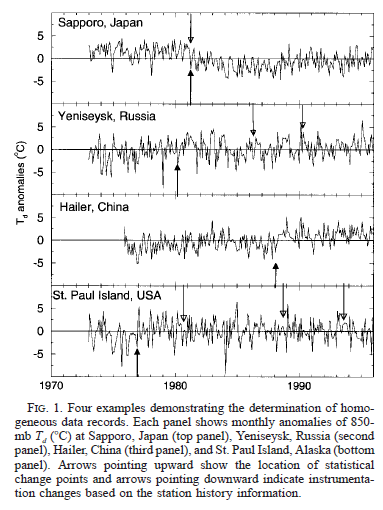
Then they have a section discussing various data homogeneity issues, which includes this graphic showing the challenge of identifying instrument changes which affect measurements:

Figure 1

They comment:

These examples show that the combination of historical and statistical information can identify some known instrument changes. However, we caution that the separation of artificial (e.g., instrument changes) and natural variability is inevitably somewhat subjective. For instance, the same instrument change at one station may not show as large an effect at another location or time of day..

Furthermore, the ability of the statistical method to detect abrupt changes depends on the variability of the record, so that the same effect of an instrument change could be obscured in a very noisy record. In this case, the same change detected at one station may not be detected at another station containing more variability.

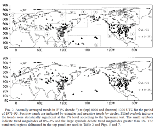
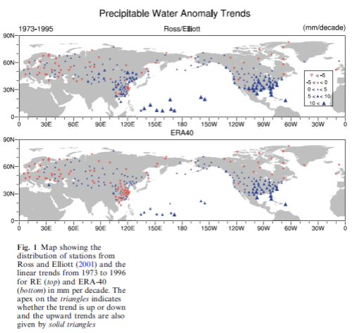
Here are their results from 1973-1995 in geographical form. Triangles are positive trends, circles are negative trends. You also get to see the distribution of radiosondes, as each marker indicates one station:

Figure 2

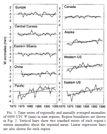
And their summary of time-based trends for each region:

Figure 3

In their summary they make some interesting comments:

We found that a global estimate could not be made because reliable records from the Southern Hemisphere were too sparse; thus we confined our analysis to the Northern Hemisphere. Even there, the analysis was limited by continual changes in instrumentation, albeit improvements, so we were left with relatively few records of total precipitable water over the era of radiosonde observations that were usable.

Emphasis added.

Well, I recommend that readers take the time to read the whole paper for themselves to understand the quality of work that has been done – and learn more about the issues with the available data.

What is Special about 1973?

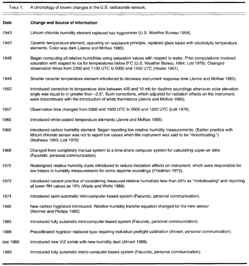
In their 1991 paper, Elliot and Gaffen showed that pre-1973 radiosonde measurements came with much more problems than post-1973.

Figure 4 – Click for larger view

Note that the above is just for the US radiosonde network.

 Our findings suggest caution is appropriate when using the humidity archives or interpreting existing water vapor climatologies so that changes in climate not be confounded by non-climate changes.

And one extract to give a flavor of the whole paper:

The introduction of the new hygristor in 1980 necessitated a new algorithm.. However, the new algorithm also eliminated the possibility of reports of humidities greater than 100% but ensured that humidities of 100% cannot be reported in cold temperatures. The overall effect of these changes is difficult to ascertain. The new algorithm should have led to higher reported humidities compared to the older algorithm, but the elimination of reports of very high values at cold temperatures would act in the opposite sense.

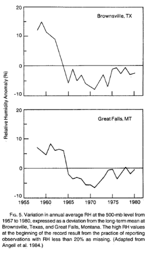
And a nice example of another change in radiosonde measurement and reporting practice. The change below is just an artifact of low humidity values being reported after a certain date:

Figure 5

As the worst cases came before 1973, most researchers subsequently reporting on water vapor trends have tended to stick to post-1973 (or report on that separately and add caveats to pre-1973 trends).

But it is important to understand that issues with radiosonde measurements are not confined to pre-1973.

Here are a few more comments, this time from Elliott in his 1995 paper:

Most (but not all) of these changes represent improvements in sensors or other practices and so are to be welcomed. Nevertheless they make it difficult to separate climate changes from changes in the measurement programs..

Since then, there have been several generations of sensors and now sensors have much faster response times. Whatever the improvements for weather forecasting, they do leave the climatologist with problems. Because relative humidity generally decreases with height slower sensors would indicate a higher humidity at a given height than today’s versions (Elliott et al., 1994).

This effect would be particularly noticeable at low temperatures where the differences in lag are greatest. A study by Soden and Lanzante (submitted) finds a moist bias in upper troposphere radiosondes using slower responding humidity sensors relative to more rapid sensors, which supports this conjecture. Such improvements would lead the unwary to conclude that some part of the atmosphere had dried over the years.

And Gaffen, Elliott & Robock (1992) reported that in analyzing data from 50 stations from 1973-1990 they found instrument changes that created “inhomogeneities in the records of about half the stations”

Satellite Demonstration

Different countries tend to use different radiosondes, have different algorithms and have different reporting practices in place.

The following comparison is of upper tropospheric water vapor. As an aside this has a focus because water vapor in the upper atmosphere disproportionately affects top of atmosphere radiation – and therefore the radiation balance of the climate.

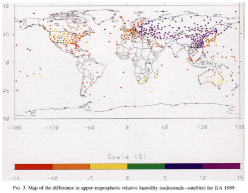
From Soden & Lanzante (1996), the data below, of the difference between satellite and radiosonde measurements, identifies a significant problem:

Figure 6

Since the same satellite is used in the comparison at all radiosonde locations, the satellite measurements serve as a fixed but not absolute reference. Thus we can infer that radiosonde values over the former Soviet Union tend to be systematically moister than the satellite measurements, that are in turn systematically moister than radiosonde values over western Europe.

However, it is not obvious from these data which of the three sets of measurements is correct in an absolute sense. That is, all three measurements could be in error with respect to the actual atmosphere..

..However, such a satellite [calibration] error would introduce a systematic bias at all locations and would not be regionally dependent like the bias shown in fig. 3 [=figure 6].

They go on to identify the radiosonde sensor used in different locations as the likely culprit. Yet, as various scientists comment in their papers, countries take on a new radiosonde in piecemeal form, sometimes having a “competitive supply” situation where 70% is from one vendor and 30% from another vendor. Other times radiosonde sensors are changed across a region over a period of a few years. Inter-comparisons are done, but inadequately.

Soden and Lanzante also comment on spatial coverage:

Over data-sparse regions such as the tropics, the limited spatial coverage can introduce systematic errors of 10-20% in terms of the relative humidity. This problem is particularly severe in the eastern tropical Pacific, which is largely void of any radiosonde stations yet is especially critical for monitoring interannual variability (e.g. ENSO).

Before we move onto reanalyses, a summing up on radiosondes from the cautious William P. Elliot (1995):

Thus there is some observational evidence for increases in moisture content in the troposphere and perhaps in the stratosphere over the last 2 decades. Because of limitations of the data sources and the relatively short record length, further observations and careful treatment of existing data will be needed to confirm a global increase.

Reanalysis – or Filling in the Blanks

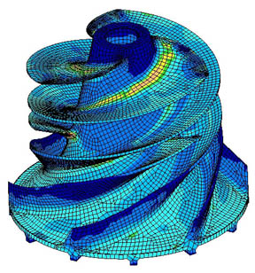
Weather forecasting and climate modelling is a form of finite element analysis (and see Wikipedia). Essentially in FEA, some kind of grid is created – like this one for a pump impellor:

Figure 7

– and the relevant equations can be solved for each boundary or each element. It’s a numerical solution to a problem that can’t be solved analytically.

Weather forecasting and climate are as tough as they come. Anyway, the atmosphere is divided up into a grid and in each grid we need a value for temperature, pressure, humidity and many other variables.

To calculate what the weather will be like over the next week a value needs to be placed into each and every grid. And just one value. If there is no value in the grid the program can’t run and there’s nowhere to put two values.

By this massive over-simplification, hopefully you will be able to appreciate what a reanalysis does. If no data is available, it has to be created. That’s not so terrible, so long as you realize it:

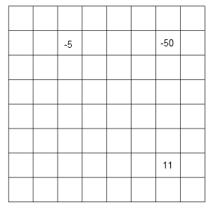
Figure 8

This is a simple example where the values represent temperatures in °C as we go up through the atmosphere. The first problem is that there is a missing value. It’s not so difficult to see that some formula can be created which will give a realistic value for this missing value. Perhaps the average of all the values surrounding it? Perhaps a similar calculation which includes values further away, but with less weighting.

With some more meteorological knowledge we might develop a more sophisticated algorithm based on the expected physics.

The second problem is that we have an anomaly. Clearly the -50°C is not correct. So there needs to be an algorithm which “fixes” it. Exactly what fix to use presents the problem.

If data becomes sparser then the problems get starker. How do we fill in and correct these values?

Figure 9

It’s not at all impossible. It is done with a model. Perhaps we know surface temperature and the typical temperature profile (“lapse rate”) through the atmosphere. So the model fills in the blanks with “typical climatology” or “basic physics”.

But it is invented data. Not real data.

Even real data is subject to being changed by the model..

NCEP/NCAR Reanalysis Project

There are a number of reanalysis projects. One is the NCEP/NCAR project (NCEP = National Centers for Environmental Prediction, NCAR = National Center for Atmospheric Research).

Kalnay (1996) explains:

The basic idea of the reanalysis project is to use a frozen state-of-the-art analysis/forecast system and perform data assimilation using past data, from 1957 to the present (reanalysis).

The NCEP/NCAR 40-year reanalysis project should be a research quality dataset suitable for many uses, including weather and short-term climate research.

An important consideration is explained:

An important question that has repeatedly arisen is how to handle the inevitable changes in the observing system, especially the availability of new satellite data, which will undoubtedly have an impact on the perceived climate of the reanalysis. Basically the choices are a) to select a subset of the observations that remains stable throughout the 40-year period of the reanalysis, or b) to use all the available data at a given time.

Choice a) would lead to an reanalysis with the most stable climate, and choice b) to an analysis that is as accurate as possible throughout the 40 years. With the guidance of the advisory panel, we have chosen b), that is, to make use of the most data available at any given time.

What are the categories of output data?

• A = analysis variable is strongly influenced by observed data and hence it is in the most reliable class
• B = although there are observational data that directly affect the value of the variable, the model also has a very strong influence on the value
• C = there are no observations directly affecting the variable, so that it is derived solely from the model fields

Humidity is in category B.

Interested people can read Kalnay’s paper. Reanalysis products are very handy and widely used. Those with experience usually know what they are playing around with. Newcomers need to pay attention to the warning labels.

Comparing Reanalysis of Humidity

Bengtsson et al (2004) reviewed another reanalysis project, ERA-40. They provide a good example of how incorrect trends can be introduced (especially the 2nd paragraph):

A bias changing in time can thus introduce a fictitious trend without being eliminated by the data assimilation system. A fictitious trend can be generated by the introduction of new types of observations such as from satellites and by instrumental and processing changes in general. Fictitious trends could also result from increases in observational coverage since this will affect systematic model errors.

Assume, for example, that the assimilating model has a cold bias in the upper troposphere which is a common error in many general circulation models (GCM). As the number of observations increases the weight of the model in the analysis is reduced and the bias will correspondingly become smaller. This will then result in an artificial warming trend.

Bengtsson and his colleagues analyze tropospheric temperature, IWV and kinetic energy.

ERA-40 does have a positive trend in water vapor, something we will return to. The trend from ERA-40 for 1958-2001 is +0.41 mm/decade, and for 1979-2001 = +0.36 mm/decade. They note that NCEP/NCAR has a negative trend of -0.24 mm/decade from 1958-2001 and -0.06mm/decade  for 1979-2001, but it isn’t a focus of their study.

They do an analysis which excludes satellite data and find a lower (but still positive) trend for IWV. They also question the magnitudes of tropospheric temperature trends and kinetic energy on similar grounds.

The point is essentially that the new data has created a bias in the reanalysis.

Their conclusion, following various caveats about the scale of the study so far:

Returning finally to the question in the title of this study an affirmative answer cannot be given, as the indications are that in its present form the ERA40 analyses are not suitable for long-term climate trend calculations.

However, it is believed that there are ways forward as indicated in this study which in the longer term are likely to be successful. The study also stresses the difficulties in detecting long term trends in the atmosphere and major efforts along the lines indicated here are urgently needed.

So, onto Trends and variability in column-integrated atmospheric water vapor by Trenberth, Fasullo & Smith (2005). This paper is well worth reading in full.

For years before 1996, the Ross and Elliott radiosonde dataset is used for validation of European Centre for Medium-range Weather Forecasts (ECMWF) reanalyses ERA-40. Only the special sensor microwave imager (SSM/I) dataset from remote sensing systems (RSS) has credible means, variability and trends for the oceans, but it is available only for the post-1988 period.

Major problems are found in the means, variability and trends from 1988 to 2001 for both reanalyses from National Centers for Environmental Prediction (NCEP) and the ERA-40 reanalysis over the oceans, and for the NASA water vapor project (NVAP) dataset more generally. NCEP and ERA-40 values are reasonable over land where constrained by radiosondes.

Accordingly, users of these data should take great care in accepting results as real.

Here’s a comparison of Ross & Elliott (2001) [already shown above] with ERA-40:

Figure 10 – Click for a larger image

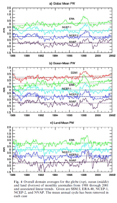
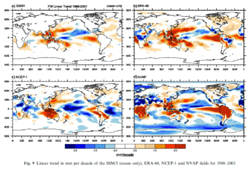
Then they consider 1988-2001, the reason being that 1988 was when the SSMI (special sensor microwave imager) data over the oceans became available (more on the satellite data later).

Figure 11

At this point we can see that ERA-40 agrees quite well with SSMI (over the oceans, the only place where SSMI operates), but NCEP/NCAR and another reanalysis product, NVAR, produce flat trends.

Now we will take a look at a very interesting paper: The Mass of the Atmosphere: A Constraint on Global Analyses, Trenberth & Smith (2005). Most readers will probably not be aware of this comparison and so it is of “extra” interest.

The total mass of the atmosphere is in fact a fundamental quantity for all atmospheric sciences. It varies in time because of changing constituents, the most notable of which is water vapor. The total mass is directly related to surface pressure while water vapor mixing ratio is measured independently.

Accordingly, there are two sources of information on the mean annual cycle of the total mass and the associated water vapor mass. One is from measurements of surface pressure over the globe; the other is from the measurements of water vapor in the atmosphere.

The main idea is that other atmospheric mass changes have a “noise level” effect on total mass, whereas water vapor has a significant effect. As measurement of surface pressure is a fundamental meteorological value, measured around the world continuously (or, at least, continually), we can calculate the total mass of the atmosphere with high accuracy. We can also – from measurements of IWV – calculate the total mass of water vapor “independently”.

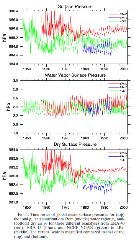
Subtracting water vapor mass from total atmospheric measured mass should give us a constant – the “dry atmospheric pressure”. That’s the idea. So if we use the surface pressure and the water vapor values from various reanalysis products we might find out some interesting bits of data..

Figure 12

In the top graph we see the annual cycle clearly revealed. The bottom graph is the one that should be constant for each reanalysis. This has water vapor mass removed via the values of water vapor in that reanalysis.

Pre-1973 values show up as being erratic in both NCEP and ERA-40. NCEP values show much more variability post-1979, but neither is perfect.

The focus of the paper is the mass of the atmosphere, but is still recommended reading.

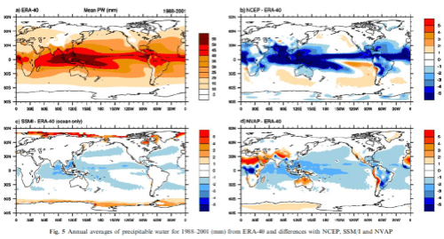
Here is the geographical distribution of IWV and the differences between ERA-40 and other datasets (note that only the first graphic is trends, the following graphics are of differences between datasets):

Figure 13 – Click for a larger image

The authors comment:

The NCEP trends are more negative than others in most places, although the patterns appear related. Closer examination reveals that the main discrepancies are over the oceans. There is quite good agreement between ERA-40 and NCEP over most land areas except Africa, i.e. in areas where values are controlled by radiosondes.

There’s a lot more in the data analysis in the paper. Here are the trends from 1988 – 2001 from the various sources including ERA-40 and SSMI:

Figure 14 – Click for a larger view

• SSMI has a trend of +0.37 mm/decade.
• ERA-40  has a trend of +0.70mm/decade over the oceans.
• NCEP has a trend of -0.1mm/decade over the oceans.

To be Continued..

As this article is already pretty long, it will be continued in Part Two, which will include Paltridge et al (2009), Dessler & Davis (2010) and some satellite measurements and papers.

Update – Part Two is published

References

On the Utility of Radiosonde Humidity Archives for Climate Studies, Elliot & Gaffen, Bulletin of the American Meteorological Society (1991)

Relationships between Tropospheric Water Vapor and Surface Temperature as Observed by Radiosondes, Gaffen, Elliott & Robock, Geophysical Research Letters (1992)

Column Water Vapor Content in Clear and Cloudy Skies, Gaffen & Elliott, Journal of Climate (1993)

On Detecting Long Term Changes in Atmospheric Moisture, Elliot, Climate Change (1995)

Tropospheric Water Vapor Climatology and Trends over North America, 1973-1993, Ross & Elliot, Journal of Climate (1996)

An assessment of satellite and radiosonde climatologies of upper-tropospheric water vapor, Soden & Lanzante, Journal of Climate (1996)

The NCEP/NCAR 40-year Reanalysis Project, Kalnay et al, Bulletin of the American Meteorological Society (1996)

Radiosonde-Based Northern Hemisphere Tropospheric Water Vapor Trends, Ross & Elliott, Journal of Climate (2001)

An analysis of satellite, radiosonde, and lidar observations of upper tropospheric water vapor from the Atmospheric Radiation Measurement Program, Soden et al,  Journal of Geophysical Research (2005)

The Radiative Signature of Upper Tropospheric Moistening, Soden et al, Science (2005)

The Mass of the Atmosphere: A Constraint on Global Analyses, Trenberth & Smith, Journal of Climate (2005)

Trends and variability in column-integrated atmospheric water vapor, Trenberth et al, Climate Dynamics (2005)

Can climate trends be calculated from reanalysis data? Bengtsson et al, Journal of Geophysical Research (2005)

Trends in middle- and upper-level tropospheric humidity from NCEP reanalysis data, Paltridge et al, Theoretical Applied Climatology (2009)

Trends in tropospheric humidity from reanalysis systems, Dessler & Davis, Journal of Geophysical Research (2010)