In Wonderland, Radiative Forcing and the Rate of Inflation we looked at the definition of radiative forcing and a few concepts around it:
- why the instantaneous forcing is different from the adjusted forcing
- what adjusted forcing is and why it’s a more useful concept
- why the definition of the tropopause affects the value
- GCM results usually don’t use radiative forcing as an input
In this article we will look at some results using the Wonderland model.
Remember the Wonderland model is not the earth. But the same is also true of “real” GCMs with geographical boundaries that match the earth as we know it. They are not the earth either. All models have limitations. This is easy to understand in principle. It is challenging to understand in the specifics of where the limitations are, even for specialists – and especially for non-specialists.
What the Wonderland model provides is a coarse geography with earth-like layout of land and ocean, plus of course, physics that follows the basic equations. And using this model we can get a sense of how radiative forcing is related to temperature changes when the same value of radiative forcing is applied via different mechanisms.
In the 1997 paper I think that Hansen, Sato & Ruedy did a decent job of explaining the limitations of radiative forcing, at least as far as the Wonderland climate model is able to assist us with that understanding. Remember as well that, in general, results we see from GCMs do not use radiative forcing. Instead they calculate from first principles – or parameterized first principles.
Doubling CO2
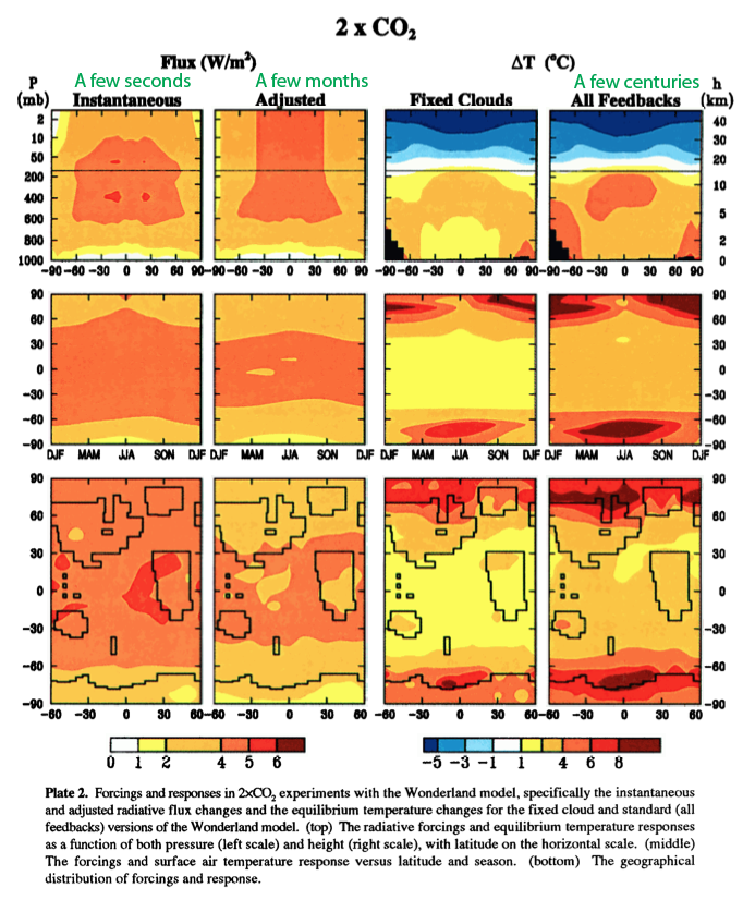
Now there’s a lot in this first figure, it can be a bit overwhelming. We’ll take it one step at a time. We double CO2 overnight – in Wonderland – and we see various results. The left half of the figure is all about flux while the right half is all about temperature:
From Hansen et al 1997
Figure 1 – Green text added – Click to Expand
On the top line, the first two graphs are the net flux change, as a function of height and latitude. First left – instantaneous; second left – adjusted. These two cases were explained in the last article.
The second left is effectively the “radiative forcing”, and we can see that the above the tropopause (at about 200 mbar) the net flux change with height is constant. This is because the stratosphere has come into radiative balance. Refer to the last article for more explanation. On the right hand side, with all feedbacks from this one change in Wonderland, we can see the famous predicted “tropospheric hot spot” and the cooling of the stratosphere.
We see in the bottom two rows on the right the expected temperature change :
- second row – change in temperature as a function of latitude and season (where temperature is averaged across all longitudes)
- third row – change in temperature as a function of latitude and longitude (averaged annually)
It’s interesting to see the larger temperature increases predicted near the poles. I’m not sure I really understand the mechanisms driving that. Note that the radiative forcing is generally higher in the tropics and lower at the poles, yet the temperature change is the other way round.
Increasing Solar Radiation by 2%
Now let’s take a look at a comparison exercise, increasing solar radiation by 2%.
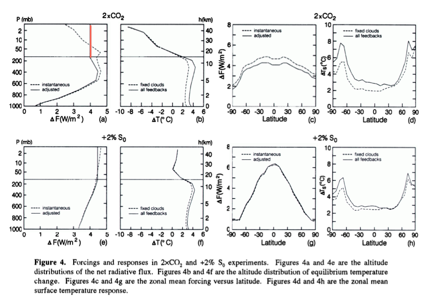
The responses to these comparable global forcings, 2xCO2 & +2% S0, are similar in a gross sense, as found by previous investigators. However, as we show in the sections below, the similarity of the responses is partly accidental, a cancellation of two contrary effects. We show in section 5 that the climate model (and presumably the real world) is much more sensitive to a forcing at high latitudes than to a forcing at low latitudes; this tends to cause a greater response for 2xCO2 (compare figures 4c & 4g); but the forcing is also more sensitive to a forcing that acts at the surface and lower troposphere than to a forcing which acts higher in the troposphere; this favors the solar forcing (compare figures 4a & 4e), partially offsetting the latitudinal sensitivity.
We saw figure 4 in the previous article, repeated again here for reference:
From Hansen et al (1997)
Figure 2
In case the above comment is not clear, absorbed solar radiation is more concentrated in the tropics and a minimum at the poles, whereas CO2 is evenly distributed (a “well-mixed greenhouse gas”). So a similar average radiative change will cause a more tropical effect for solar but a more even effect for CO2.
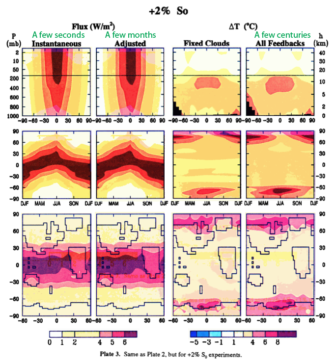
We can see that clearly in the comparable graphic for a solar increase of 2%:
From Hansen et al (1997)
Figure 3 – Green text added – Click to Expand
We see that the change in net flux is higher at the surface than the 2xCO2 case, and is much more concentrated in the tropics.
We also see the predicted tropospheric hot spot looking pretty similar to the 2xCO2 tropospheric hot spot (see note 1).
But unlike the cooler stratosphere of the 2xCO2 case, we see an unchanging stratosphere for this increase in solar irradiation.
These same points can also be seen in figure 2 above (figure 4 from Hansen et al).
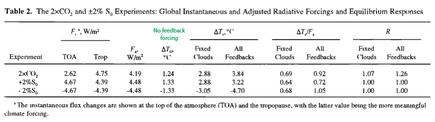
Here is the table which compares radiative forcing (instantaneous and adjusted), no feedback temperature change, and full-GCM calculated temperature change for doubling CO2, increasing solar by 2% and reducing solar by 2%:
From Hansen et al 1997
Figure 4 – Green text added – Click to Expand
The value R (far right of table) is the ratio of the predicted temperature change from a given forcing divided by the predicted temperature change from the 2% increase in solar radiation.
Now the paper also includes some ozone changes which are pretty interesting, but won’t be discussed here (unless we have questions from people who have read the paper of course).
“Ghost” Forcings
The authors then go on to consider what they call ghost forcings:
How does the climate response depend on the time and place at which a forcing is applied? The forcings considered above all have complex spatial and temporal variations. For example, the change of solar irradiance varies with time of day, season, latitude, and even longitude because of zonal variations in ground albedo and cloud cover. We would like a simpler test forcing.
We define a “ghost” forcing as an arbitrary heating added to the radiative source term in the energy equation.. The forcing, in effect, appears magically from outer space at an atmospheric level, latitude range, season and time of day. Usually we choose a ghost forcing with a global and annual mean of 4 W/m², making it comparable to the 2xCO2 and +2% S0 experiments.
In the following table we see the results of various experiments:

Hansen et al (1997)
Figure 5 – Click to Expand
We note that the feedback factor for the ghost forcing varies with the altitude of the forcing by about a factor of two. We also note that a substantial surface temperature response is obtained even when the forcing is located entirely within the stratosphere. Analysis of these results requires that we first quantify the effect of cloud changes. However, the results can be understood qualitatively as follows.
Consider ΔTs in the case of fixed clouds. As the forcing is added to successively higher layers, there are two principal competing effects. First, as the heating moves higher, a larger fraction of the energy is radiated directly to space without warming the surface, causing ΔTs to decline as the altitude of the forcing increases. However, second, warming of a given level allows more water vapor to exist there, and at the higher levels water vapor is a particularly effective greenhouse gas. The net result is that ΔTs tends to decline with the altitude of the forcing, but it has a relative maximum near the tropopause.
When clouds are free to change the surface temperature change depends even more on the altitude of the forcing (figure 8). The principal mechanism is that heating of a given layer tends to decrease large-scale cloud cover within that layer. The dominant effect of decreased low-level clouds is a reduced planetary albedo, thus a warming, while the dominant effect of decreased high clouds is a reduced greenhouse effect, thus a cooling. However, the cloud cover, the cloud cover changes and the surface temperature sensitivity to changes may depend on characteristics of the forcing other than altitude, e.g. latitude, so quantitive evaluation requires detailed examination of the cloud changes (section 6).
Conclusion
Radiative forcing is a useful concept which gives a headline idea about the imbalance in climate equilibrium caused by something like a change in “greenhouse” gas concentration.
GCM calculations of temperature change over a few centuries do vary significantly with the exact nature of the forcing – primarily its vertical and geographical distribution. This means that a calculated radiative forcing of, say, 1 W/m² from two different mechanisms (e.g. ozone and CFCs) would (according to GCMs) not necessarily produce the same surface temperature change.
References
Radiative forcing and climate response, Hansen, Sato & Ruedy, Journal of Geophysical Research (1997) – free paper
Notes
Note 1: The reason for the predicted hot spot is more water vapor causes a lower lapse rate – which increases the temperature higher up in the troposphere relative to the surface. This change is concentrated in the tropics because the tropics are hotter and, therefore, have much more water vapor. The dry polar regions cannot get a lapse rate change from more water vapor because the effect is so small.
Any increase in surface temperature is predicted to cause this same change.
With limited research on my part, the idealized picture of the hotspot as shown above is not actually the real model results. The top graph is the “just CO2” graph, and the bottom graph is the “CO2 + aerosols” – the second graph is obviously closer to the real case:
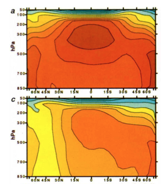
From Santer et al 1996
Many people have asked for my comment on the hot spot, but apart from putting forward an opinion I haven’t spent enough time researching this topic to understand it. From time to time I do dig in, but it seems that there are about 20 papers that need to be read to say something useful on the topic. Unfortunately many of them are heavy in stats and my interest wanes.


