In Part Seven we had a look at a 2008 paper by Gettelman & Fu which assessed models vs measurements for water vapor in the upper troposphere.
In this article we will look at a 2010 paper by Chung, Yeomans & Soden. This paper studies outgoing longwave radiation (OLR) vs temperature change, for clear skies only, in three ways (and comparing models and measurements):
- by region
- by season
- year to year
Why is this important and what is the approach all about?
Let’s suppose that the surface temperature increases for some reason. What happens to the total annual radiation emitted by the climate system? We expect it to increase. The hotter objects are the more they radiate.
If there is no positive feedback in the climate system then for a uniform global 1K (=1ºC) increase in surface & atmospheric temperature we expect the OLR to increase by 3.6 W/m². This is often called, by convention only, the “Planck feedback”. It refers to the fact that an increased surface temperature, and increased atmospheric temperature, will radiate more – and the “no feedback value” is 3.6 W/m² per 1K rise in temperature.
To explain a little further for newcomers.. with the concept of “no positive feedback” an initial 1K surface temperature rise – from any given cause – will stay at 1K. But if there is positive feedback in the climate system, an initial 1K surface temperature rise will result in a final temperature higher than 1K.
If the OLR increases by less than 3.6 W/m² the final temperature will end up higher than 1K – positive feedback. If the OLR increases by more than 3.6 W/m² the final temperature will end up lower than 1K – negative feedback.
Base Case
At the start of their paper they show the calculated clear-sky OLR change as the result of an ideal case. This is the change in OLR as a result of the surface and atmosphere increasing uniformly by 1K:
- first, from the temperature change alone
- second, from the change in water vapor as a result of this temperature change, assuming relative humidity stays constant
- finally, from the first and second combined
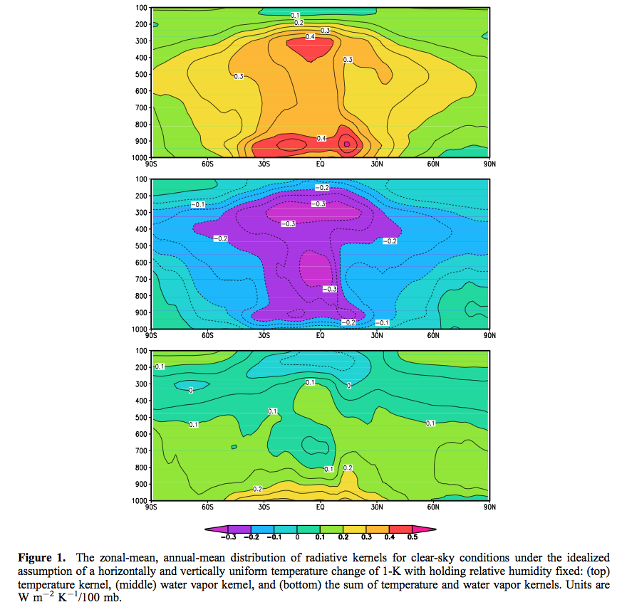
From Chung et al (2010)
Figure 1 – Click to expand
The graphs show the breakdown by pressure (=height) and latitude. 1000mbar is the surface and 200mbar is approximately the tropopause, the place where convection stops.
The sum of the first graph (note 1) is the “no feedback” response and equals 3.6 W/m². The sum of the second graph is the “feedback from water vapor” and equals -1.6 W/m². The combined result in the third graph equals 2.0 W/m². The second and third graphs are the result if relative humidity is constant.
We can also see that the tropics is where most of the changes take place.
They say:
One striking feature of the fixed-RH kernel is the small values in the tropical upper troposphere, where the positive OLR response to a temperature increase is offset by negative responses to the corresponding vapor increase. Thus under a constant RH- warming scenario, the tropical upper troposphere is in a runaway greenhouse state – the stabilizing effect of atmospheric warming is neutralized by the increased absorption from water vapor. Of course, the tropical upper troposphere is not isolated but is closely tied to the lower tropical troposphere where the combined temperature-water vapor responses are safely stabilizing.
To understand the first part of their statement, if temperatures increase and overall OLR does not increase at all then there is nothing to stop temperatures increasing. Of course, in practice, the “close to zero” increase in OLR for the tropical upper troposphere under a temperature rise can’t lead to any kind of runaway temperature increase. This is because there is a relationship between the temperatures in the upper troposphere and the lower- & mid- troposphere.
Relative Humidity Stays Constant?
Back in 1967, Manabe & Wetherald published their seminal paper which showed the result of increases in CO2 under two cases – with absolute humidity constant and with relative humidity constant:
Generally speaking, the sensitivity of the surface equilibrium temperature upon the change of various factors such as solar constant, cloudiness, surface albedo, and CO2 content are almost twice as much for the atmosphere with a given distribution of relative humidity as for that with a given distribution of absolute humidity..
..Doubling the existing CO2 content of the atmosphere has the effect of increasing the surface temperature by about 2.3ºC for the atmosphere with the realistic distribution of relative humidity and by about 1.3ºC for that with the realistic distribution of absolute humidity.
They explain important thinking about this topic:
Figure 1 shows the distribution of relative humidity as a function of latitude and height for summer and winter. According to this figure, the zonal mean distributions of relative humidity closely resemble one another, whereas those of absolute humidity do not. These data suggest that, given sufficient time, the atmosphere tends to restore a certain climatological distribution of relative humidity responding to the change of temperature.
It doesn’t mean that anyone should assume that relative humidity stays constant under a warmer world. It’s just likely to be a more realistic starting point than assuming that absolute humidity stays constant.
I only point this out for readers to understand that this idea is something that has seemed reasonable for almost 50 years. Of course, we have to question this “reasonable” assumption. How relative humidity changes as the climate warms or cools is a key factor in determining the water feedback and, therefore, it has had a lot of attention.
Results From the Paper
The observed rates of radiative damping from regional, seasonal, and interannual variations are substantially smaller than the rate of Planck radiative damping (3.6W/m²), yet slightly larger than that anticipated from a uniform warming, constant-RH response (2.0 W/m²).
The three comparison regressions can be seen, with ERBE data on the left and model results on the right:
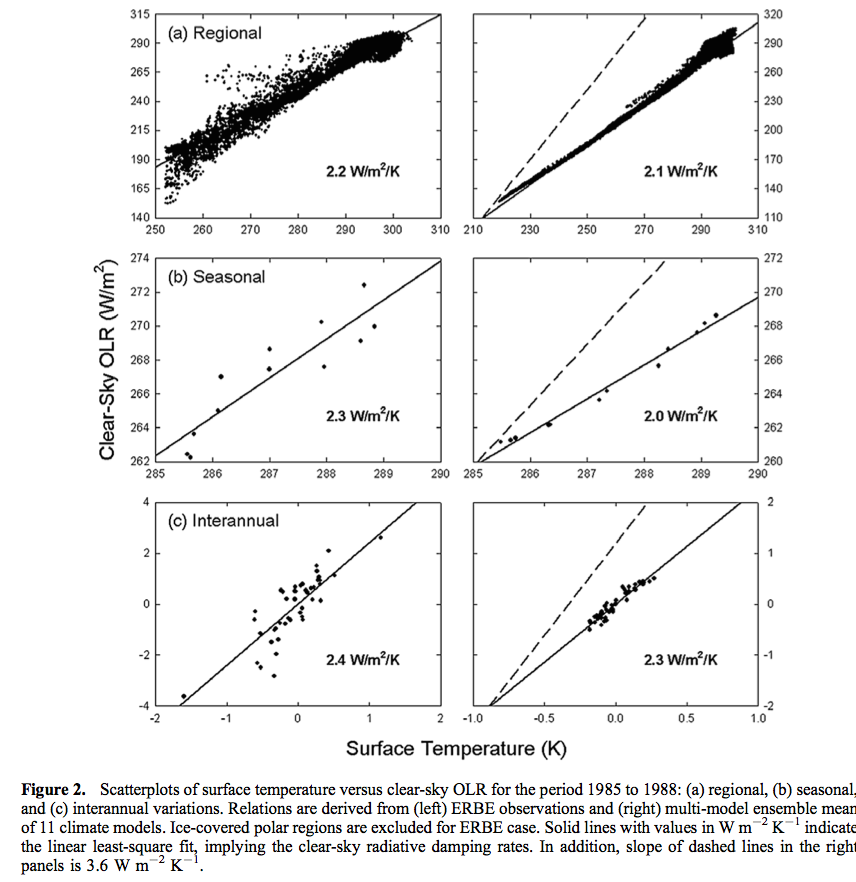
From Chung et al (2010)
Figure 2 – Click to expand
In the next figure, the differences between the models can be seen, and compared with ERBE and CERES results. The red “Planck” line is the no-feedback line, showing that (for these sets of results) models and experimental data show a positive feedback (when looking at clear sky OLR).
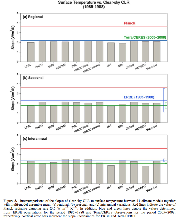
From Chung et al (2010)
Figure 3 – Click to expand
Conclusion
At the least, we can see that climate models and measured values are quite close, when the results are aggregated. Both the model and the measured results are a long way from neutral feedback (the dashed slope in figure 2 and the red line in figure 3), instead they show positive feedback, quite close to what we would expect from constant relative humidity. The results indicate that relative humidity declines a little in the warmer case. The results also indicate that the models calculate a little more positive feedback than the real world measurements under these cases.
What does this mean for feedback from warming from increased GHGs? It’s the important question. We could say that the results tell us nothing, because how the world warms from increasing CO2 (and other GHGs) will change climate patterns and so seasonal, regional and year to year changes in periods from 1985-1988 and 2005-2008 are not particularly useful.
We could say that the results tell us that water vapor feedback is demonstrated to be a positive feedback, and matches quite closely the results of models. Or we could say that without cloudy sky data the results aren’t very interesting.
At the very least we can see that for current climate conditions under clear skies the change in OLR as temperature changes indicates an overall positive feedback, quite close to constant relative humidity results and quite close to what models calculate.
The ERBE results include the effect of a large El Nino and I do question whether year to year changes (graph c in figs 2 & 3) under El Nino to La Nino changes can be considered to represent how the climate might warm with more CO2. If we consider how the weather patterns shift during El-Nino to La Nina it has long been clear that there are positive feedbacks, but also the weather patterns end up back to normal (the cycle ends). I welcome knowledgeable readers explaining why El Nino feedback patters are relevant to future climate shifts, perhaps this will help me to clarify my thinking, or correct my misconceptions.
However, the CERES results from 2005-2008 don’t include the effect of a large El Nino and they show an overall slightly more positive feedback.
I asked Brian Soden a few question about this paper and he was kind enough to respond:
Q. Given the much better quality data since CERES and AIRS, why is ERBE data the focus?
A. At the time, the ERBE data was the only measurement that covered a large ENSO cycle (87/88 El Nino event followed by 88/89 La Nina)
Q. Why not include cloudy skies as well in this review? Collecting surface temperature data is more challenging of course because it needs a different data source. Is there a comparable study that you know of for cloudy skies?
A. The response of clouds to surface temperature changes is more complicated. We wanted to start with something relatively simple; i.e., water vapor. Andrew Dessler at Texas AM has a paper that came out a few years back that looks at total-sky fluxes and thus includes the effects on clouds.
Q. Do you know of any studies which have done similar work with what must now be over 10 years of CERES/AIRS.
A. Not off-hand. But it would be useful to do.
Articles in the Series
Part One – introducing some ideas from Ramanathan from ERBE 1985 – 1989 results
Part One – Responses – answering some questions about Part One
Part Two – some introductory ideas about water vapor including measurements
Part Three – effects of water vapor at different heights (non-linearity issues), problems of the 3d motion of air in the water vapor problem and some calculations over a few decades
Part Four – discussion and results of a paper by Dessler et al using the latest AIRS and CERES data to calculate current atmospheric and water vapor feedback vs height and surface temperature
Part Five – Back of the envelope calcs from Pierrehumbert – focusing on a 1995 paper by Pierrehumbert to show some basics about circulation within the tropics and how the drier subsiding regions of the circulation contribute to cooling the tropics
Part Six – Nonlinearity and Dry Atmospheres – demonstrating that different distributions of water vapor yet with the same mean can result in different radiation to space, and how this is important for drier regions like the sub-tropics
Part Seven – Upper Tropospheric Models & Measurement – recent measurements from AIRS showing upper tropospheric water vapor increases with surface temperature
Part Eight – Clear Sky Comparison of Models with ERBE and CERES – a paper from Chung et al (2010) showing clear sky OLR vs temperature vs models for a number of cases
Part Nine – Data I – Ts vs OLR – data from CERES on OLR compared with surface temperature from NCAR – and what we determine
Part Ten – Data II – Ts vs OLR – more on the data
References
An assessment of climate feedback processes using satellite observations of clear-sky OLR, Eui-Seok Chung, David Yeomans, & Brian J. Soden, GRL (2010) – free paper
Thermal equilibrium of the atmosphere with a given distribution of relative humidity, Manabe & Wetherald, Journal of the Atmospheric Sciences (1967) – free paper
Notes
Note 1: The values are per 100 mbar “slice” of the atmosphere. So if we want to calculate the total change we need to sum the values in each vertical slice, and of course, because they vary through latitude we need to average the values (area-weighted) across all latitudes.


Two remarks.
(1) Chung, Yeomans & Soden [2010] use ERA40 surface temperatures. However, ERA40 surface temperatures are known to have considerable biases in surface temperatures (in particular over cold areas). See:
https://www.mpimet.mpg.de/fileadmin/static/era40/result.htm
To what extent that is relevant for the analysis I don’t know, but some care has to be taken with for example the interpretation of their figure 2 (is the observed relation Tsurf vs OLR really linear?).
(2) To some extent this comes back to (1), in particular figure 2c, left panel. I don’t think that the fit to the points is fair, it looks like the two outlier points at approximately -1.7C and +1.2C disturb the fit. I’m not sure which type of linear fitting they did (can’t find it in the paper), but it appears to have been a standard ordinary linear regression.
However, this type of linear fitting is problematic if your distribution of points is non-Guassian (= not randomly distributed). And this appears to be the case. Just by visual inspection, if I were to remove these two points then it appears that the fit to the points could be much steeper and easily be close to 3.6 W/K.
It has be long known and well established in statistical literature that linear fitting can be problematic, there are plenty of methods and algorithms around to circumvent these problems. I hope the authors don’t mind me saying this, but it is a bit disturbing/disappointing that this has escaped the referees and that it is not addressed.
So, is the relation Tsurf vs OLR really that consistent with model results – in particular on longer time scales? Based on these results I am not convinced.
Or am I missing something here?
Cheers, Jos.
Jos,
If ERA40 has a bias which is an offset, e.g. too cold in the arctic, then it wouldn’t affect the calculation of slope.
The later CERES data used NCEP/NCAR reanalysis.
I’m interested in trying to do some CERES analysis myself. I did make a start quite a while ago but there is a bit of a mountain to climb before you can get started. Of course I got diverted on other climate interests.
I have dug out my old notes and will see if I can get any time to extract relevant data.
SoD,
Your link to the Chung et al paper does not work, it’s probably either temporary or valid only for you. This link
http://onlinelibrary.wiley.com/wol1/doi/10.1029/2009GL041889/full
is likely to work better.
Your post does not define the radiative kernel that’s shown in Figure 1. I don’t think that the concept is not obvious enough to everyone. Chung et al defines it by:
Then a minor remark. Looking at graphics like Figure 1, it’s worthwhile to notice that half of the Earth area is between 30S and 30N, and only 13.4% at higher latitudes than 60 degrees. The Arctic and Antarctic areas cover only 6.0%, if we put the limit at 70 degrees. One of the unrealistic features of Figure 1 is the latitudinal uniformity of the warming, but from the relatively small area of the polar regions follows that Arctic amplification has less overall influence than one might think.
Thanks Pekka, I just updated the article.
For the tropics, at the upper tropospheric levels, figure 1[bottom] indicates negative radiative kernel values which would indicate cooling. Positive radiative kernel values at the surface mean a decrease in static stability of the tropics are imposed by heating and humidifying as for a constant RH.
I have found something similar by using CFS 1 by 1 analysis data, including clouds. With this atmosphere, I calculated radiance changes for condition of 2xCO2 with heated ( by 2.4K ), humidified ( as for constant RH ), and heated & humidified. The result is for destabilizing the troposphere, which leads to heat and humidity aloft -> which leads to destabilizing again, -> which leads to heat and humidity aloft -> … ( ad infinitum )
One aspect of this is as follows: The tropopause is modeled to encounter no temperature change due to global warming. Thus a constant relative humidity for the atmosphere at the tropopause will have no change in humidity. Subsidence of this air to lower levels ( such as the top of the maritime inversion in the subtropics ) means no change in relative humidity there either. It might be that for these paths, constant absolute humidity prevails while for other areas, constant relative humidity occurs.
It may be this process, or it may be totally unrelated, but the IPCC did indicate this – areas of decreasing humidity and areas of increasing humidity, subject to all the usual doubts and caveats ( see Figure a. ):
SOD: The uniform 1 degK increase in temperature in Figure 1 is an unrealistic scenario because of lapse rate feedback. Feedbacks are calculated in terms of W/m2/K, where K is surface temperature. A 1 K rise in surface temperature will be associated with more than a 1 K rise in the upper troposphere, making the increase in OLR larger than shown. This could eliminate the runaway greenhouse effect seen in Figure 1c.
Why is Planck feedback 3.6 W/m2/K in this paper and 3.3 W/m2/K in Part 1 (Ramanathan) and 3.2 W/m2/K elsewhere? (There is no citation associated with the value Soden uses.) According to the IPCC, the no-feedbacks climate sensitivity for 2XCO2 is 1.15 K. If the forcing from 2XCO2 is 3.7 W/m2 (at tropopause), I calculate a Planck feedback (PF) of 3.2 W/m2/K. If the forcing is 3.5 W/m2 at the TOA, PF is 3.04 W/m2. If you treat the earth as a blackbody at 255 K, then a 1 degK increase is a 3.76 W/m2 increase (from 240 W/m2). If you treat the earth as a gray body at 290 degK, a 1 degK rise is 3.3 W/m2. (I prefer this reasoning.) Table 9.5 from AR5 WG1, says models exhibit a Planck feedback from 3.1-3.3 W/m2. Are any of the values more appropriate than any other?
Frank,
Chung et al write referring to their model calculations presented in Figure 1.:
Thus the value 3.6 W/m^2/K is not a value claimed to apply to the real world, but to their calculation with all it’s assumptions (clear sky, uniform warming by 1 K without change in absolute humidity).
Pekka: On the graphs, there are green and blue lines for Ceres and Erbe observations of the real world. The exact location of the Planck feedback red line in the real world is important for calculating ECS. The accuracy with which these models of the real world match observations of the real world (not some uniformly warming world) is important. The artificial situation that yielded 3.6 W/m2/K seems out of place here (though useful for raising ECS).
My understanding is that the Figure 1(top) tells about the distribution of the Planck response between contributions from different parts of the atmosphere. What’s missing from that figure, and what’s not shown anywhere in the paper is the contribution of the surface to the radiative kernel.
As we case is a clear sky case the contribution of the surface is large and dominating at higher latitudes. In tropics the humidity is so high that even the clear sky transmits only a small fraction of the IR emitted from the surface, but at higher latitudes that fraction is very significant.
SoD’s radiative transfer model could be used to study these effects. Using different model atmospheres as input it should be possible to reproduce results similar to those of Figure 1, but getting all the smaller details requires that a large number of detailed atmospheric profiles are available.
SOD wrote: “We could say that the results tell us that water vapor feedback is demonstrated to be a positive feedback, and matches quite closely the results of models.”
Speaking cynically, we could conclude that it is possible to tune your climate model so that OLR from clear skies is in agreement with observations by ERBE. Soden has regional data. It would be interesting to see if models can reproduce regional variation in the strength of WV+LR feedback
Frank,
Reproducing the clear sky WV feedback can be done reliably given good data on the state of the atmosphere. Every reasonably carefully constructed model should give essentially the same results from the same input profiles. The definition of the WV feedback is such that the results are correct essentially by definition as long as technical errors have not been made.
Lapse rate feedback is even more trivial to calculate, when the atmospheric profiles of cases to compare are given as fixed input.
The real problems originate in the generation of the atmospheric profiles, not in the calculation of the feedbacks from given profiles. Cloud feedbacks are well known to be an even bigger problem.
Pekka wrote: “Reproducing clear sky WV [and LR] feedback can be done reliably given good data on the state of the atmosphere.”
Agreed. But the AOGCM first needs to get the state of the atmosphere correct. Getting a global average for WV+LR feedback to agree with observation by tuning a parameter may be possible, so reproducing regional variation in such feedback is a much more meaningful challenge. NH vs SH. Tropics vs subtropics vs temperate vs sub arctic. Ocean vs land. Soden has regional data, but he isn’t discussing it here. Held has discussed why model relative humidity in the boundary layer over oceans must rise with SST. Is this what CERES observes?
As Feynman writes in Cargo Cult Science, it is important to distinguish between two types of agreement between theory and observations. Sometimes theories are constructed to explain certain observations. In those cases, agreement between theory and observation provides negligible confirmation the theory is correct. Sometimes a theory constructed to fit certain observations turns out to explain other observations, or better still, prompts new experiments which agree with the theory. In those cases, agreement provides important confirmation.
An AOGCM with an incorrect albedo can not possibly reproduce GMST, so cloud parameters are tuned until outgoing SWR agrees with observations. Agreement between observed and predicted reflected SWR provides no validation. I don’t know if models are tuned so that clear sky OLR agrees with observations (producing no useful confirmation) or if this agreement is meaningful (because it wasn’t the result of tuning). Unless model developers explain how their models are tuned, the agreement isn’t validation.
Two points which may be of interest,
1. Outside CliSci, Planck radiation describes black-body radiation for which a material-independent function describes spectral intensities of emission spectra. This is not the function for thermal radiation observed in OLR spectra. Nitpicking perhaps, but the difference reflects an entropy increase and free energy dissipation as an energy flux transits the troposphere, i.e. weather. 240W @280K is not equivalent to 240W @210K!
2. The Planck radiation sensitivity is 4W/T and close to what is observed. Suppose, instead, that OLR is proportional to the difference in temperature across the troposphere. The sensitivity is then W/delta T and numerically identical for the parameters used above. This is the default description for all other dissipative processes: electrical, viscous, diffusive, chemical. (Actually fluxes are often assumed proportional to gradients adding a factor of two.)
From IPCC:

The global average indicates an increase in (absolute column) humidity.
Interestingly,
1.) large areas exhibit a decrease in humidity, thus radiating more energy.
2.) the polar regions exhibit also exhibit a decrease in humidity which is contrary to an understood cause of ‘Arctic Amplification’.
Turbulent Eddie,
The regional temperature changes over that period are not necessarily positive either.
Here’s an extract from IPCC AR5 ch 2:
I haven’t done any kind of comparison other than looking at the two graphs but there does seem to be a relationship for colder areas and reduced water vapor.
This is what we should be expecting because most of the water vapor (by mass) is in the boundary layer and sea surface temp and boundary layer humidity have a strong relationship. It’s less certain what happens above the boundary layer (as explained in earlier articles in this series) – which is unfortunately where the radiation effects are most important for feedback.
Zhu et al (2007) found that cloud formation for ENSO and for global warming have different characteristics and are the result of different physical mechanisms. The change in low cloud cover in the 1997-1998 El Niño came mainly as a decrease in optically thick stratocumulus and stratus cloud. The decrease is negatively correlated to local SST anomalies, especially in the eastern tropical Pacific, and is associated with a change in convective activity. ‘During the 1997–1998 El Niño, observations indicate that the SST increase in the eastern tropical Pacific enhances the atmospheric convection, which shifts the upward motion to further south and breaks down low stratiform clouds, leading to a decrease in low cloud amount in this region. Taking into account the obscuring effects of high cloud, it was found that thick low clouds decreased by more than 20% in the eastern tropical Pacific… In contrast, most increase in low cloud amount due to doubled CO2 simulated by the NCAR and GFDL models occurs in the subtropical subsidence regimes associated with a strong atmospheric stability.’
There is an increased loss of energy in the tropics in El Nino – and decrease d losses in La Nina – in net SW and IR effects. The global effect in IR is more muted but there – and the cloud effect changes sign between the tropics and subtropics. The 2008 period shows less IR losses in the tropics and more in the sub-tropics with less cloud cover and decreased cloud height. The effects are hugely variable between ENSO events.
As in Zhu et al above – you have to wonder whether ENSO is any sort of an analogy for warming.
riellison,
Likewise I wonder about ENSO for giving us valuable information on climate feedback for global warming (as I mentioned in the article).
A paper that suggests something similar: Water vapor and cloud feedback over the tropical oceans: Can we use ENSO as a surrogate for climate change? Lau, Ho & Chu, GRL (1996):
A more recent paper that perhaps thinks feedback from ENSO is a reasonable approach (I infer that from the paper but I’m not sure): Estimates of the Water Vapor Climate Feedback during El Nino–Southern Oscillation, Dessler & Wong, Journal of Climate (2009):
http://www.esrl.noaa.gov/psd/enso/mei/
ENSO originates in the upwelling zone of the eastern equatorial Pacific. It involves more or less upwelling of cold subsurface water – something that varies not just in 2 to 5 year ENSO cycles but over decades to millennia. The feedbacks include changes in surface temperature – which by the physical fact of warmer air holding more moisture influences specific humidity. Not surprising therefore that warmer air in EL Nino holds more moisture. There is of course other feedbacks – cloud, currents, wind, tropical upwelling – that collectively result in the increased planetary cooling from the tropics in El Nino.
Multi-decadal variability in the Pacific is defined as the Interdecadal Pacific Oscillation (e.g. Folland et al,2002, Meinke et al, 2005, Parker et al, 2007, Power et al, 1999) – a proliferation of oscillations it seems. The latest Pacific Ocean climate shift in 1998/2001 is linked to increased flow in the north (Di Lorenzo et al, 2008) and the south (Roemmich et al, 2007, Qiu, Bo et al 2006)Pacific Ocean gyres. Roemmich et al (2007) suggest that mid-latitude gyres in all of the oceans are influenced by decadal variability in the Southern and Northern Annular Modes (SAM and NAM respectively) as wind driven currents in baroclinic oceans (Sverdrup, 1947). see more at – http://watertechbyrie.com/2014/06/23/the-unstable-math-of-michael-ghils-climate-sensitivity/
Greenhouse gases in the atmosphere have a fundamental different dynamic. It adds to warmth in the atmosphere – but whether or not the atmosphere actually warms depends on the collective behaviour of the climate system. Which shifts more or less radically every 20 or 30 years. If surface temperatures actually warm – which seems unlikely for at least a decade more – then we can happily accept that increased water vapour in the atmosphere is a trivial result in the midst of much complexity.
On another topic – you may be interested in – http://watertechbyrie.com/2015/05/05/the-devils-of-ecomodernism/ – while I can’t begin to draw conclusions on climate science the policy response to small anthropogenic pressures in a chaotic system need to be on a human scale and meet human needs.
“Or we could say that without cloudy sky data the results aren’t very interesting.”
Yes, and probably not of any practical use. Moreover, it looks like the plots of surface temperature to OLR fluxes are just linear regressions, no?
“At the very least we can see that for current climate conditions under clear skies the change in OLR as temperature changes indicates an overall positive feedback, quite close to constant relative humidity results and quite close to what models calculate.”
But again is very unlikely to be of any use in determining the net combined effect of clouds and water vapor, because clear vs. cloudy skies are constantly changing. That the water vapor feedback is positive in clear sky conditions is trivially true. The net combined feedback of clouds is determined by the ratios of incremental reflection from clouds to incremental IR opacity of clouds, and which is the greater or the dominate effect on the planet.
The plot here of about 3 decades worth of satellite measurements shows — at least from a long term macroscopic perspective, that incremental reflection of clouds exceeds their IR opacity for the bulk of the planet:
That is, the data simply shows, independent of causation, that above about 0C, the more clouds there are the cooler it tends to be, and the fewer clouds there are the warmer it tends to be.
Only when the surface temperature is below about 0C is the net effect of clouds to warm. That is, below about 0C when there are more clouds it tends to be warmer and when there are fewer clouds it tends to be cooler.
The fundamental physics behind this are above about 0C, the surface is mostly likely snow and ice free, so the net effect of clouds is to cool the surface by reflecting more solar power away than is delayed by the clouds. Below about 0C, the surface is most likely snow and/or ice covered. Snow and ice are roughly as reflective to solar energy as clouds are, thus about the same amount of solar energy is reflected whether there are clouds or no clouds. Clouds are much more opaque to upwelling IR from the surface and lower atmosphere than the clear sky is, so the net effect of clouds is warm the surface by delaying more solar energy than is reflected away in total. And of course, if there is no Sun, the same applies because clouds are better IR absorbers than the clear sky.
For reference, here is water vapor or water content from the same data set.
It shows unambiguously that increased surface temperatures increases water vapor as predicted. Note though the relationship becomes less and less the as the data goes towards and finally into the tropics. The surface temperature saturates around 300K. Meaning regardless of how much more water content, the surface temperature doesn’t further rise. Note how this saturation occurs at roughly the same place in the first plot where the cloud coverage starts to increase again as data goes into the tropics.
The fundamental physical mechanism(s) behind this is beyond a certain temperature there is so much water being evaporated, removing so much heat from the surface (as the latent heat of evaporation), providing so much ‘fuel’ (i.e. water) for cloud formation, that the combination of cloud caused (from solar reflection) and evaporative caused cooling overwhelms any increase in atmospheric IR opacity from increased water vapor.
This analysis supports that the net negative feedback of clouds and water vapor is strongest in the tropics and then gets progressively weaker as you head out of the tropics toward the poles (and even becomes net positive once the surface becomes snow and/or ice covered).
*For the satellite data plots, each small dot represents a monthly average for one grid area in a 2.5 degree slice of latitude. The green and blue dots are the 25 year averages for each 2.5 degree slice of latitude (1983-2008). From right to left, it goes from the tropics to the poles. The data is from ISCCP and processed this source here: http://www.palisad.com/co2/sens/index.html
BTW, this analysis of the data I’ve outlined is completely consistent with the results Lindzen is getting looking at tropical data (and then extrapolating to the poles) in his latest 2011 paper with Choi, where they get a fairly strong net negative feedback in the tropics which then becomes weaker when ‘shared’ over the globe.
RW,
It’s not possible to conclude much from your first figure. Both the surface temperature and the amount of clouds depend on the location. A typical observation is that the highest day-time temperatures are obtained in arid low-latitude locations like Sahara. Relatively cool nights prevent very high average temperatures, but these areas contribute to the points that represent high temperatures and low cloudiness. The reasons for the presence of such areas are not those that you discuss.
The importance of such additional factors means that it’s impossible to tell whether the observations provide any support for your interpretation or not. More detailed analysis is required for that.
“Both the surface temperature and the amount of clouds depend on the location.”
I certainly agree with this. There is nothing in the plot that indicates why the cloud coverage is what it is in a particular hemisphere or grid area. That’s determined by a number of factors no doubt. While the first plot of surface temperature to cloud amount doesn’t establish causation in either direction or indicate why the cloud coverage is what it is in any one area, it does establish that above about 0C when there are more clouds on monthly average per grid area, it tends to be cooler, and when there are fewer clouds, it tends to be warmer. Note this relationship becomes even more pronounced as you get closer and closer to the tropics where eventually water saturation occurs around 300K. Where as, below about 0C, when there are more clouds, it tends to be warmer, and when there are fewer clouds it tends to be cooler.
The critical question for CO2 induced global warming is what will the combined net effect of clouds and water vapor be on incremental warming? That is, will their combined effect or response be to reduce the warming or further increase the warming?
It’s agreed that the net radiative effect of clouds is to cool by about 20 W/m^2 on global average, right? Considering clouds are significantly more opaque to IR than the clear sky, i.e. GHGs by themselves, that’s a super strong cooling effect. What that 20 W/m^2 really means is that clouds on global average reflect about 20 W/m^2 more of incident solar energy back out to space than is delayed or ‘trapped’ by them.
This further means there are basically two ways in which the cloud response will enhance the warming. By letting more solar energy in via reduced clouds or further delaying the release of absorbed solar energy via increased clouds trapping more solar energy than they reflect back out to space. The former seems highly unlikely because warming causes more water to evaporate, which provides more fuel for cloud cover.
Where as, there is really only one way that clouds will act to reduce the warming, and that is via increased clouds where their incremental solar reflection exceeds their incremental increase in IR opacity.
The next critical question is how do you determine the direction of causation for temperature changes to cloud changes? If you’re looking at global average data, the surface temperature changes are super small and the SW feedback in particular (due to random changes in cloud coverage), is or least can theoretically be very noisy. That is, are the clouds changes mostly causing the temperature changes (forcing) or are the temperature changes mostly causing the clouds changes (feedback).
By looking at the hemispheres separately, there is no difficulty in determining cause and effect for temperature changes to clouds changes, because it’s overwhelmingly obvious the cloud changes are not causing the measured temperature changes. The temperature changes are of course caused by the large swings in incident solar energy that occur throughout the year.
These plots here are what establish causation for temperature changes to cloud changes (again 25 year averages from the same data set):
Note how as the incoming solar energy increases, the gain decreases below the average, and as the incoming solar energy decreases, the gain increases above the average. The gain being out of phase with the input energy source (in this case post albedo solar power) is the signature of a system that is controlled by net negative feedback. That is, the gain decreasing as the input power source increases (and vice versa). Climate sensitivity as it’s conventionally defined can be fully quantified by dimensionless gain and has the exact same physical meaning.
Now, also note how as the incoming solar energy increases, the cloud coverage increases, and as the incoming solar energy decreases, the cloud coverage decreases. Note how in both hemispheres the average surface temperature stays well above 0C. This suggests the fundamental mechanism that maintains the energy balance appears to be that, on global average, increasing cloud coverage causing cooling (more solar energy is reflected than is delayed) and decreasing cloud coverage causes warming (more solar energy is absorbed than exits to space). Or that in the aggregate, when clouds are increasing, the surface is too warm and trying to cool, and when clouds are decreasing, the surface is too cool and trying to warm. That is, these counter balancing mechanisms dynamically maintain the energy balance.
This analysis of the data supports that the net negative feedback of clouds and water vapor is strongest in the tropics and then gets progressively weaker as you head out of the tropics toward the poles (and even becomes net positive once the surface becomes snow and/or ice covered). This is totally consistent with the results Lindzen is getting. That is, he is getting a very strong net negative feedback in the tropics, which is then necessarily weakened when ‘shared’ with the whole Earth to arrive at his global feedback factor estimate. Lindzen even acknowledges there may be other feedbacks operating outside the tropics, but that the tropics are the dominant feedback effect on the planet since that is where most of the solar energy arrives.
When you consider that the vast majority of energy from the Sun arrives in the area of about 23N to 23S, i.e. the tropics, and the least amount arrives in the area of above 63N and below 63S, i.e. the frigid zone, where much of the surface is snow and/or ice covered, it’s of little consequence that the net effect radiative effect of clouds is to warm in these areas.
Sorry, those last two paragraphs should have said the following:
“….This is totally consistent with the results Lindzen is getting. That is, he is getting a very strong net negative feedback in the tropics, which is then necessarily weakened when ‘shared’ with the whole Earth to arrive at his global feedback factor estimate. Lindzen even acknowledges there may be other non-negative feedbacks operating outside the tropics, but that the tropics are the dominant feedback effect on the planet since that is where most of the solar energy arrives.
When you consider that the vast majority of energy from the Sun arrives in the area of about 23N to 23S, i.e. the tropics, and the least amount arrives in the area of above 63N and below 63S, i.e. the frigid zone, where much of the surface is snow and/or ice covered, it’s of little consequence that the net effect radiative of clouds is to warm in these areas.”
RW,
What you say about the role of clouds in areas covered by snow is largely true, but that’s also an example of the logical error that you make, when you interpret that the observation supports Lindzen’s hypothesis. When you present similar arguments also about the influence of desert areas, moist tropics, various parts of oceans, etc., you should observe that nothing obvious is left that would tell anything about the validity of the iris hypothesis (nothing in support of it, nothing against it, simply nothing).
Are these figures published? I’m studying the water vapor and surface temperature relationship in the Arctic, and these figures provide useful context for my observations.
Pekka,
I still have a really long reply post to you in the moderators que just before that last correction post.
“What you say about the role of clouds in areas covered by snow is largely true, but that’s also an example of the logical error that you make, when you interpret that the observation supports Lindzen’s hypothesis. When you present similar arguments also about the influence of desert areas, moist tropics, various parts of oceans, etc., you should observe that nothing obvious is left that would tell anything about the validity of the iris hypothesis (nothing in support of it, nothing against it, simply nothing).”
How are you deriving that? I understand Lindzen’s IRIS hypothesis is not that of a reduction in overall cloudiness, but instead a reduction in cirrus clouds. His hypothesis may or may not be correct, but it seems perfectly consistent with the physics I have laid out.
I was saying that the physics I laid out is consistent with the results of Lindzen and Choi 2011. His feedback factor of about 0.7C per 3.7 W/m^2 is the same as what the author here is deriving: http://www.palisad.com/co2/sens/index.html
Note that the absolute gain or ‘zero-feedback’ gain of the system is about 1.6 (i.e. 385/239 = 1.61). 0.7C per 3.7 W/m^2 results in about 3.6 W/m^2 of additional net surface gain, which means the incremental gain of the system is very close to unity. Or that each 1 W/m^2 forcing results in about 1 W/m^2 of post feedback net surface gain:
An incremental post feedback gain of 1.0 is lower than the absolute gain of 1.6, indicating net negative feedback. Note that a sensitivity of +3.3C requires an incremental gain of 4.8. That is, +3.3C equals about +18 W/m^2 of net surface gain and 18/3.7 = 4.8.
RW,
I wrote that the data you present does not either support or refute the iris hypothesis. That means that iris hypothesis is consistent with the data, but so are very many conflicting hypotheses.
“I wrote that the data you present does not either support or refute the iris hypothesis. That means that iris hypothesis is consistent with the data, but so are very many conflicting hypotheses.”
I agree with this, but you can layer on as much complexity as you want and/or derive as many hypothesis from that complexity as you want. But there is no inherent reason that doing so is necessary or enhances our understanding of the fundamental questions and issues involved in accurately calculating climate sensitivity. Occam’s razor has long been one of science’s best logical tools.
I agree some of the explanations and derivations I presented almost seem too simplistic to be correct, but it doesn’t mean they are wrong. Or that more complex explanations and derivations are right.
“I still have a really long reply post to you in the moderators que just before that last correction post.”
It looks like it went through. Maybe you saw it. At any rate, I think the author makes a pretty compelling case that L&C are getting it right and the consensus purported sensitivity of 3.3C is way off.
Further note that the consensus sensitivity of 3.3C requires an incremental gain 3x greater than the absolute gain of 1.6 (i.e. 4.8/1.6 = 3), yet the data shows the exact opposite behavior that would be consistent with that:
That is, as the incident post albedo solar energy increases above the global averge, the gain decreases below the global average. Note also that in the second graph, Lindzen’s sensitivity estimate is well inside the range of the measured data, where as the sensitivity estimate supported by the IPCC lies far outside the range of data.
If you really think a sensitivity of 3.3C is feasible (or even possible), you might explain why it doesn’t take 1162 W/m^2 of net surface gain (over 100C!) to offset the 239 W/m^2 of incident forcing from the Sun, i.e. (18/3.7)*239 = 1162.
BTW, the techniques the author is using are those one would use to reverse engineer an unknown but measurable system. The author is following the protocol used in standard systems analysis, where as climate science seems to have kind of made up its own rules regarding how feedback and sensitivity are quantified (yet kept the control theory implications associated with feedback and sensitivity established in standard systems analysis).
In standard systems analysis, sensitivity to some forcing or stimuli is quantified as dimensionless power densities ratios or more specifically as output power divided by input power. In the case of the climate, the output power is about 385 W/m^2 of surface radiation per S-B and in the input power is about 239 W/m^2 of radiation entering the system from the Sun. The output power of the system is 385 W/m^2 and not 485 W/m^2, because 385 W/m^2 is the net amount or actual amount of power input to the surface after all other sources of power, radiant and non-radiant, in excess of 385 W/m^2 entering and leaving the surface, have already had their effect on the net amount of input at the surface/atmosphere boundary.
When sensitivity is quantified as degrees C per watt of forcing, it obscures the non-linearity of the system’s response to post albedo solar input, which is necessary to see in order to accurately quantify the incremental response of the system to a change the energy balance, such as increased GHGs.
Can we at least agree that the net feedback comes down to whether the net incremental effect of clouds is to cool or warm? That is, unless you are one who believes that clouds will decrease in response to warming? Or at least decrease in areas that receive more Sun.
[…] last article we looked at a paper which tried to unravel – for clear sky only – how the OLR […]
[…] in OLR would be negative feedback and a smaller increase would be positive feedback (e.g. see Part Eight with the plot of OLR changes vs latitude and height, which integrated globally gives 3.6 […]
I’ve been interested in the various estimates for Planck feedback and no-feedbacks climate sensitivity. I’m asking the question here, because I can’t find a more appropriate post.
This post mentions a value of 3.6 W/m2/K. The standard Figure used by climate scientists is -3.21 W/m2 from Soden and Held 2006 and is derived from experiments with the GFDL model wherein a control run was halted at various time points, the temperature temporarily raised everywhere by 1 K, and the change in OLR was calculated by the model. (Info from the GFDL model was then applied to output from 13 other models,)
A simpler model is to treat the Earth as a blackbody at 255 with an emissivity of 1. Differentiating the S-B law with respect to temperature gives dW/dT = -4oT^3 = -3.76 W/m2/K.
Assuming the climate model is correct, our planet emits like a blackbody at 255 K (240 W/m2), but exhibits a Planck feedback like a blackbody at 242 K (3.21 W/m2/K), a non-trivial discrepancy. I understand that average (T^n) is bigger than (average T)^n for this situation and explored models with multiple emitting layers that emit a total of 240 W/m2 as well as models that have emissivity less than one. None were satisfying. (IIRC, a single layer with a temperature around 300 K and a very low emissivity fits the data perfectly and 288 K and e = 0.61 is close. But no location behaves this way.) Things get more complicated if one allows emissivity to vary with temperature when differentiating, which adds a oT^4*(de/dT) term. I suppose I should differentiate Planck’ Law and then integrate over all wavelengths to see if that makes a difference.
I’ver hear rumors that the 1 K rise used by S&H was 1 K in terms of GMST, but weighted towards polar regions where more warming is expected. S&H 2006 doesn’t say that, but their cited earlier method is behind a paywall.
Does anyone understand why our planet emits like a blackbody at 255 K (240 W/m2), but exhibits a Planck feedback like a blackbody at 242 K (3.21 W/m2/K)?
Frank,
What do you mean by ‘Planck feedback’?
The so-called Planck response of about +3.3 W/m^2 at the TOA per 1C of surface warming is just based on linearly warming according to the lapse rate. This is what the field considers to be the ‘no-feedback’ response measure at the TOA. For 1C it’s about 3.3 W/m^2 and for 1.1C it’s about 3.6 W/m^2.
I don’t know what you’re asking.
I’m unaware of a difference between Planck response and Planck feedback. IMO, both terms refer to the tendency of all things – including our planet as a whole – to emit more thermal radiation when they warm.
If a feedback is an component of our climate that varies with surface temperature and effects radiative balance at the TOA, then Planck response is a feedback. If so, “no-feedbacks” means no feedbacks besides Planck feedback.
Frank,
The Earth does not emit like a blackbody at 255K. It emits the same total amount of energy, but the spectrum is not a blackbody spectrum by any stretch of the imagination. The brightness temperature varies a lot with frequency. Then there’s the problem that the Earth is not isothermal either. That means the temperature averaged over the surface will always be lower than for an isothermal body emitting the same amount of energy. A climate model would take this into account while a simple blackbody model wouldn’t.
DeWitt,
You are correct, but I don’t see how that answers Frank’s question. Consider half the emission as a blackbody at 280 K and half at 220 K. The average T is 250 K but the effective emission T (from the 4th root of the mean of T^4) is 255.2 K. The average feedback (from the cube root of the mean of T^3) is 253.5 K. In the right direction, but way too small a difference. I don’t see how you can get the feedback T down to 242 K as long as the temperature change is everywhere the same.
DeWitt: The Earth is not a blackbody. The objective is to find as simple a model for the Earth as possible that emits 240 W/m2 and has a Planck feedback of 3.2 W/m2/K. Such a model might “explain” Soden and Held’s result for Planck feedback. I’ve tried many, including the one mentioned by Mike: 50% BB at 220 K and 50% BB at 270 K. I believe that you can partition the planet up into as many zones and temperatures as you want and won’t be able to find a BB model that does this.
If you introduce an emissivity term, you can solve for two equations and two unknowns. eoT^4 = 240 and 4eoT^3 = 3.21. T = 299 and e = 0.53. Not a great model: where on the planet is the emissivity 0.53? The temperature is 299 some places, but those places don’t emit many photons that reach space.
However, your reply had an interesting suggestion. Let’s suppose our model emits like a BB at some % of wavelengths and doesn’t emit anything at the other wavelengths. If 53% of wavelengths emit like at BB at 299 K and the rest emit nothing, we get 240 W/m2 and 3.2 W/m2/K.
Now let’s try something reasonable:
10% BB at 288 for all wavelengths,
+ 90% BB at 265 K for 80% of wavelengths,
+ 90% at 265 K with zero absorption cross-section for 20% of wavelengths
Result: 240 W/m2. 3.58 W/m2/K.
10% BB at 288 for all wavelengths,
+ 90% BB at 274 K for 70% of wavelengths,
+ 90% at 274 K with zero absorption cross-section for 30% of wavelengths
Result: 240 W/m2. 3.48 W/m2/K.
It is really hard to get Planck feedback as low as 3.2 W/m2.
Frank,
I’ve got an idea of what might be going on. The Planck feedback is for a uniform 1 K increase in temperature. But I think that applies only in the troposphere. If 15% of emission to space is from the stratosphere and stratospheric temperature does not change, then you get the calculated Planck feedback, which is 85% of that expected at 255 K. But increased CO2 causes stratospheric temperature to go down, since that is a purely radiative effect it may be included in the model calculation of Planck feedback. Then it would take less than 15% from the stratosphere to produce the smaller feedback.
There does some to be a fair bit emitted from the stratosphere. See figure 2 at https://scienceofdoom.com/2013/01/08/visualizing-atmospheric-radiation-part-three-average-height-of-emission/.
Mike M.,
If you use MODTRAN looking up from the tropopause, defined as where the temperature starts to increase, emission from the stratosphere is less than 10W/m². The decrease in the satellite lower stratosphere temperature anomaly from 1979 to the present is about 1.5°
DeWitt wrote: “If you use MODTRAN looking up from the tropopause, defined as where the temperature starts to increase, emission from the stratosphere is less than 10W/m². The decrease in the satellite lower stratosphere temperature anomaly from 1979 to the present is about 1.5°”
Thanks. So that is about 4% from the stratosphere, which would not be enough if the stratospheric temperature stayed constant. But the temperature change is 2-3 times the tropospheric change and in the opposite direction. So that would seem to give a Planck response of 12-16%. About right if my mental math is right.
You need to drop emission from the stratosphere by about 6% to reduce the sensitivity from the simple blackbody sensitivity of 3.8 W/m²/K at 255K to 3.2. I think trying to reduce this to a simple model is a waste of time. The atmosphere isn’t isothermal or isotropic, not to mention clouds. Trying to treat it as if it were is not going to be productive.
If the S&H model calculation didn’t include CO2, which seems likely, you’re barking up the wrong tree anyway.
DeWitt,
The object here is not to reduce things to a simple model but to understand why the Planck feedback parameter is so small. Simple models are one way of trying to understand that. Saying “that’s what the models say” is not an explanation. A clear figure created from model output and showing what happens would be great, if that exists. I expect Frank would also be happy with that if someone could point us towards such a figure.
I think you are correct that the stratospheric cooling due to CO2 is probably not relevant, unlike what I supposed.
DeWitt and Mike: Soden and Held (2006) says:
http://journals.ametsoc.org/doi/full/10.1175/JCLI3799.1
“Thus, we perturb [+1 K] only the tropospheric state in the feedback computation, but we examine the response of TOA fluxes, rather than the tropopause fluxes, to these perturbations. It can be shown that this is equivalent to assuming that the net dynamical heating of the stratosphere is unchanged, and that we can ignore the response of stratospheric temperatures to the change in tropospheric temperature, water, and clouds. In our experience, it is preferable to make these simplifications rather than attempt to define changes in GCM fluxes at the tropopause; the latter are sensitive to arbitrariness in the definition of the tropopause and to the movement of the tropopause as climate changes.”
To compute Kx, we first calculate the control top-of-the-atmosphere (TOA) radiative fluxes using 3-hourly values of temperature, water vapor, cloud properties, and surface albedo from a control simulation of the GFDL GCM. For each level k, the temperature is increased by 1 K and the resulting change in TOA fluxes determines(∂R/∂Tk). Similarly, (∂R/∂wk)is computed by perturbing the water vapor in each layer by holding relative humidity constant and increasing the temperature used to compute the saturation-mixing ratio by 1 K. For (∂R/∂α), a 1% decrease in surface albedo is used to compute the TOA flux perturbation. Figure 2 displays the zonal-mean, annual-mean distribution of Kx for temperature, water vapor, and surface albedo. The reader is referred to Held and Soden (2000) for further discussion of this method and interpretation of the spatial structure of the feedback kernels.
If I’m lucky, have have pasted Figure 2 below. Note the units are W/m2/K/100 mb or W/m2/K/tenth of the atmosphere.
A BB at 255 K model might be the brightest red -0.38 W/m2/K/100 mbar everywhere?
Or it might be -0.56 W/m2/K/100 mbar at the surface and drop to about -0.20 W/m2/K at the tropopause (210 K).
I don’t understand Figure 2 and S&H 2000 is behind a paywall.
Frank,
I have also been puzzling over Figure 2 in Soden & Held 2006. It does seem to show how different regions affect the response in that redder areas produce a larger change in emission to space for a given temperature change. But I don’t understand how to quantitatively interpret it since it must account for both emission at one height and absorption above that height. S&H 2000 does not look helpful after a quick glance.
On the bottom of page 2 they say: “We define feedbacks in terms of the change in global mean surface temperature (Ts) and the change in radiative flux at the top of the atmosphere (R).” So the Planck feedback is not for a uniform 1 K change.
Top of page 3 they say “The temperature feedback can be split further as … where 0 assumes that the temperature change is uniform throughout the troposphere and L (i.e., lapse rate feedback) is the modification due to nonuniformity of the temperature change”. Which seem to contradict the earlier statement. But I think this just refers to using the same T change at all altitudes (zero lapse rate feedback) rather than at all latitudes.
On page 4 under results they say “Intermodel differences in lambda_0 arise from different spatial patterns of warming; models with greater high-latitude warming, where the temperature is colder, have smaller values of lambda_0.” So they are computing the response per K for each location then multiplying by the T change at that location for a 1 K average T change. And using a model to get the distribution of T change.
So the larger T change in colder areas weights those areas more strongly and lowers the feedback. And they keep the stratosphere temperature unchanged, so that lowers the feedback in proportion to how much emission is from the stratosphere (a few percent).
Mike: Feedback X comes from (pdR/pdX)*(pdX/pdTs). In the case of Planck feedback, X=Ts. There is only one model, the GFDL model, that the authors can use to interrupt the control run, temporarily raise the temperature of all grid cells and the surface by 1 K, calculate the increase in TOA OLR, and re-start the control run. That gives them pdR/pdTs_GFDL. For other models, the second term “must” be pdTs_GFDL/pdTs_model. But I’m not sure how this ratio is evaluated. If a 1 K increase in GMST a 2 K rise in polar regions in some models and a 3 K rise in other models, then maybe you could calculate this term for every grid cell and average.
(pdR/pdTs_GFDL)*(pdTs_GFDL/pdTs_model)
If you measure Planck feedback by raising the temperature 1 K in all grid cells, then lapse rate feedback corrects for the fact that rising absolute humidity reduces the lapse rate – meaning that 1 K of surface warming turns out to be more than 1 K in the upper troposphere. This seems straightforward to me. So I don’t expect the temperature feedback plot to include lapse rate feedback. However, those bright red areas at 300 mb (220? K) would have dW/dT of only 0.24 W/m2/K/100mb if they behaved like a blackbody.
Frank,
“I’m unaware of a difference between Planck response and Planck feedback. IMO, both terms refer to the tendency of all things – including our planet as a whole – to emit more thermal radiation when they warm.
If a feedback is an component of our climate that varies with surface temperature and effects radiative balance at the TOA, then Planck response is a feedback. If so, “no-feedbacks” means no feedbacks besides Planck feedback.”
I wouldn’t describe and characterize it like this, but I suppose this is one way to conceptualize it.
AR4 has a glossary with definitions. Their definition is much broader than mine:
“Climate feedback: An interaction mechanism between processes in the climate system is called a climate feedback when the result of an initial process triggers changes in a second process that in turn influences the initial one. A positive feedback intensifies the original process, and a negative feedback reduces it.”
The initial process is surface warming (or cooling). The second process is a change in radiative cooling to space. Planck feedback (negative) limits the amount of warming (or cooling).
A clearer example is Pinabubo. At the peak, volcanic aerosols were blocking about 3 W/m2 of incoming SWR. However, after about a year, GMST was about 0.5 K cooler. A Planck feedback of -3.2 W/m2/K would mean that radiative cooling to space would be about 1.6 W/m2 less after cooling than before. So the -3 W/m2 radiative imbalance would be reduced by the 1.6 W/m2 that was no longer escaping to space due to cooling, leaving an imbalance of only -1.4 W/m2. So the imbalance and therefore rate of cooling had dropped in half. 18 months after the eruption, incoming and outgoing radiation were in balance, even though a substantial amount of aerosol still remained in the stratosphere.
Frank,
Again, I’m not quite sure what you’re getting at here. To me, the so-called ‘Planck feedback’ refers to the inherent negative feedback that exists because as anything warms it radiates more, i.e. its rate of cooling increases. The so-called ‘Planck response’ relates to the warming that would restore balance with ‘no-feedback’ and is something that would manifest itself at the TOA. For 1C of surface warming, the ‘Planck response’ is estimated to be around 3.3 W/m^2. All it is though is linear warming according the lapse rate, which itself is quantified by the ratio of emitted surface radiation to outgoing TOA radiation. That ratio is roughly 1.6 (385/239 = 1.61), and +1C from a baseline of 287K equals about +5.3 W/m^2 of surface radiation; and 5.3/1.6 = 3.3.
Frank,
The bottom line is the field assumes that if the change in the total outgoing flux (emitted LW plus reflected SW) is greater than the so-called ‘Planck response’, it indicates net negative feedback, and if the total outgoing flux is less than the ‘Planck response’, it indicates net positive feedback. However, this assumes the changes observed at the TOA are in fact feedback in response to the surface temperature changes. Many, including so-called ‘skeptics’ like Spencer and Lindzen, have published papers showing how non-feedback cloud variations can contaminate the results.
I still don’t know what it is you’re asking or trying to get at.
Why am I not surprised.
I would love to point out how this article was very helpful in finally falsifying “climate change” – basically the whole of it. Let me briefly outline the story.
Already in part four there was this reference to Dessler et al 2008 (D08), that invalidated the “regional” proxy: “We are looking at regional variations in lapse rate in a fixed climate, rather than variations in the average lapse rate as the climate changes. This result demonstrates the unsuitability of using variations in different regions in our present climate as a proxy for climate change.”
Let me describe the problem with my own words. For these proxies to work, you will need to observe the same behaviour that is expected over long term trend of global warming. So there has to be positive water vapor feedback (WVF) and a negative lapse rate feedback (LRF). If the observed dOLR/dTs relation is smaller than the Planck Response, this would indicate a (fast) positive feedback. Today the common estimate would be WVF + LRF = 1.3, up from 0.96 in AR4 btw. So although LRF is negative, like -0.5, WVF is accordinly larger positive, like 1.8. Then for instance 1.8 – 0.5 = 1.3
What D08 points out, is that there is no negative WVF in the regional proxy, but rather a positive WVF component. You would not want to call it a positive WVF, because physically it is not a feedback response. But anyway, since Tz in the sense of the average temperature within the troposphere, warms and cools slower than Ts (by latitude), the WVF component is positive. With the above restriction of WVF + LRF = 1.3, and an LRF = +1, it solves for WVF = 0.3!!! In other words, just because you expect a negative LRF, you will wrongly asign a large positive figure to WVF.
D08 only suggests to not use the regional proxy, which kind of pulls down one pillar of the theory. However, the problem is far more systemic. The seasonal proxy is struck with the exact same issue. There too the variation of the tropospheric temperature is far smaller than that of Ts. The relation of Tz/Ts is about 0.55 for the globe and just 0.4 for the tropics (30°N – 30°S). This also falsifies the assumption of a “super GHE” in the tropics – as it is just “super sluggish” tropospheric temperature. Again there is a huge positive LRF component in the proxy that was erroneously interpreted to be positive WVF. And so goes the second pillar.
Only the interannual proxy actually has a dTz/dTs > 1 term. So that will not disqualify it as a proxy. However, something else does. As visible in the Chung et al 2010 chart above, with “(c) interannual” the spread on the x-scale extends to roughly 2.8 (-1.65 to + 1.15). Such a large spread in Ts never occurred over that period (1985-1988). The actual spread was no larger than 0.7K! The reason for this reported spread is in the clear sky sampling, where regions are counted in, or counted out, depending on wether they were clear enough. However, this approach is illicit and falsly produces a low dOLR/dTs relation. Without this issue, the regression will yield a result way larger than the Planck Response, indicating a negative feedback all over.
It is a long story with plenty of other sources of information, but to cut it short: in reality LRF is far greater than WVF, and the overall term is indeed strongly negative. In other words, water vapor is strong negative feedback. The blunder already named in D08 was really the core of the illusion of a strong WVF, that just never existed.