Once we start measuring climate parameters we get a lot of data. To compare datasets, or datasets with models, we can look at means, standard deviations, medians, percentiles, and so on.
I’ve frequently mentioned the problem that climate is nonlinear. If we investigate the underlying physics of most processes we find that the answer to the problem does not scale linearly as inputs change.
Roca et al (2012) say:
The main reason for water vapor to be of importance to the energetics of the climate lies in the nonlinearity of the radiative transfer to the humidity. The outgoing longwave radiation (OLR) is indeed much more sensitive to a given perturbation in a dry rather than moist environment, conferring a central role of the moisture distribution in these regions to the radiation budget of the planet and to the overall climate sensitivity.
The authors demonstrate that with the same mean value of water vapor in a dry climate we can get different values of radiation to space for different distributions. (Note that FTH = free tropospheric humidity. This is the humidity above the atmospheric boundary layer – the boundary layer ranges from between a few hundred meters and one km):
Energy constraints on planet Earth (i.e. applying the first law of thermodynamics) require that, at equilibrium, the Earth emits in the long wave as much radiation as its gets from the Sun. This budget approach is hence focused on the mean values of the OLR over the whole planet and over long time scales corresponding to the global radiative-convective equilibrium theory.
While the mean OLR is the constrained parameter, owing to the nonlinearity of the clear-sky radiative transfer to water vapour (Figs. 2a, 3), the whole distribution of moisture has to be considered rather than its mean in order to link the distribution of humidity to that of radiation.
To illustrate this, the OLR sensitivity to FTH curve (Fig. 2a) and four distributions of FTH for a dry case are considered (Fig. 2bc): a constant distribution with mean of 14.5%, an uniform distribution with mean of 14.5% bounded within plus or minus 5%, a Gaussian distribution with mean of 14.5% (and a 5% standard deviation) and a generalized log-normal distribution with a mean of 14.5% shown in Fig. 2c. The mean OLR corresponding to the constant distribution is 311 W/m². The uniform and normal distribution yield to a mean OLR larger by 0.7 W/m² in both cases.
The log-normal PDF, on the other hand, gives a 3 W/m² overestimation of the OLR with respect to the constant case. At the scale of the doubling of CO2 problem, such a systematic bias could be significant depending on its geographical spread, which is explored next.
PDF is the probability density function.
And in case it’s not clear what the authors were saying, the same average humidity can result in significantly different OLR depending on the distribution of the humidity from which the average was calculated.
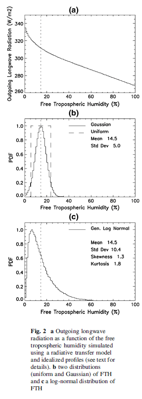
Figure 1
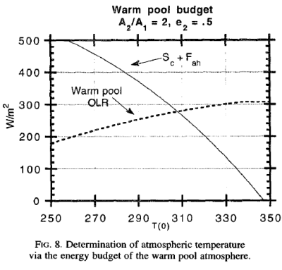
We saw the importance of the drier subsiding regions of the tropics in Clouds & Water Vapor – Part Five – Back of the envelope calcs from Pierrehumbert in that they have much higher OLR than the convective regions.
This paper calculates the results (using the vertical profile of temperature as a multi-year summer average of Bay of Bengal conditions from ERA-40) that with a constant boundary layer humidity (BLH), increasing FTH from 1% to 15% reduces OLR by 23 W/m². Increasing FTH from 35% to 50% reduces OLR by only 8 W/m². The spectral composition of these changes is interesting:
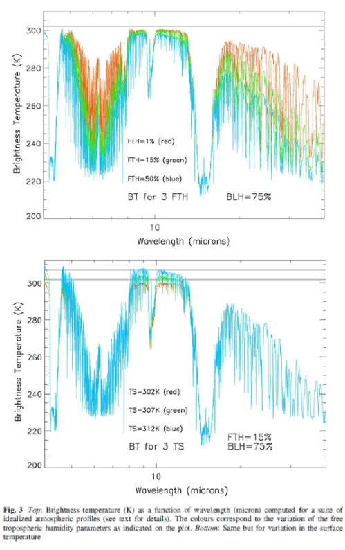
Figure 2
The authors comment that the changes in surface temperature (in the 2nd graph) result in a smaller change in OLR, which seems to be indicated from the brightness temperature graph. I have asked Remy Roca if he has the OLR calculations for this second graph to hand.
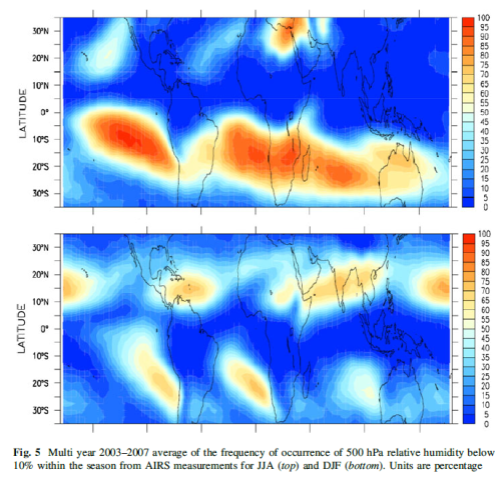
Then a statistical test is applied to values of humidity at 500 hPa (about 5.5 km altitude):

Figure 3
We see that the moist areas are more likely to have a normal (gaussian) distribution, while the dry areas are less likely.
Here is an actual distribution from Ryoo et al (2008), for different regions from 250 hPa (about 11km) for both tropical (red) and sub-tropical regions (blue):
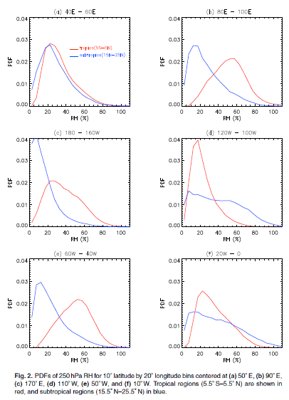
Figure 4
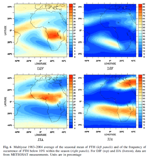
The authors use the frequency of occurrence of relative humidity less than 10% as a measure:
The need of handling the whole PDF of humidity instead of only the mean of the field implies the manipulation of the upper moments of the distribution (skewness and kurtosis). While the computations are straightforward, the comparison of two PDFs through the comparison of their 4 moments is not. Assuming a generalized log-normal distribution also requires 4 parameters to be fitted. It can be brought down to 2 parameters by imposing the lower and upper range limit of the distribution (0 and 100% for instance) at the cost of limiting the possible distributions.
The simplified model (Ryoo et al. 2009) also comprises only two parameters, linked to the first two moments of the distribution. Still, the moments-to-moments comparison of PDFs remains difficult.
Here, it is proposed to limit the analysis to a single parameter characterizing the PDF with emphasis on the dry foot of the distribution: the frequency of occurrence of RH below 10%, noted in the following as RHp10.
The paper then provides some graphs of the frequency of RH below 10%. We can think of it as another way of looking at the same data, but focusing on the drier end of the dataset:
From Roca et al 2012
Figure 5
From Roca et al 2012
Figure 6
The authors then consider the source of the driest air at 500hPa. Now this uses what is called the advection-condensation method, something I hope to cover in a later article on water vapor. But for interest, here is their result:
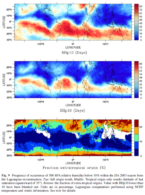
From Roca et al 2012
Figure 7
The middle graph is the first graph with air sourced from the extra-tropics excluded.
The RHp10 distribution of the reconstructed field for the boreal summer 2003 is compared to the RHp10 distribution obtained by keeping only the air masses that experienced last saturation within the intertropical belt (35S–35N) in Fig. 9. Excluding the extra-tropical last saturated air masses overall moistens the atmosphere. The domain averaged RHp10 decreases from 37 to 23% without the extra-tropical influence. While the patterns overall remain similar within the two computations, the driest areas nevertheless appear more impacted and less spread in the tropics only case (Fig. 9 middle). The very dry features in the subtropical south Atlantic is mainly built from tropical originating air with the fraction of extra-tropical influence less than 10% (Fig. 9c).
Conclusion
Even if a monthly mean value of a climatological value from a model matches the measurement monthly mean it doesn’t necessarily mean that the consequences for the climate are the same.
Small changes in the distribution of values (for the same average) can have significant impacts. Here we see that this is the case for dry regions.
In Clouds & Water Vapor – Part Five – Back of the envelope calcs from Pierrehumbert we saw that these dry regions have a big role in cooling the tropics and therefore in regulating the temperature of the planet. Understanding more about the distribution of humidity and the mechanisms and causes is essential for progress in climate science.
Articles in the Series
Part One – introducing some ideas from Ramanathan from ERBE 1985 – 1989 results
Part One – Responses – answering some questions about Part One
Part Two – some introductory ideas about water vapor including measurements
Part Three – effects of water vapor at different heights (non-linearity issues), problems of the 3d motion of air in the water vapor problem and some calculations over a few decades
Part Four – discussion and results of a paper by Dessler et al using the latest AIRS and CERES data to calculate current atmospheric and water vapor feedback vs height and surface temperature
Part Five – Back of the envelope calcs from Pierrehumbert – focusing on a 1995 paper by Pierrehumbert to show some basics about circulation within the tropics and how the drier subsiding regions of the circulation contribute to cooling the tropics
Part Six – Nonlinearity and Dry Atmospheres – demonstrating that different distributions of water vapor yet with the same mean can result in different radiation to space, and how this is important for drier regions like the sub-tropics
Part Seven – Upper Tropospheric Models & Measurement – recent measurements from AIRS showing upper tropospheric water vapor increases with surface temperature
Part Eight – Clear Sky Comparison of Models with ERBE and CERES – a paper from Chung et al (2010) showing clear sky OLR vs temperature vs models for a number of cases
Part Nine – Data I – Ts vs OLR – data from CERES on OLR compared with surface temperature from NCAR – and what we determine
Part Ten – Data II – Ts vs OLR – more on the data
References
Tropical and Extra-Tropical Influences on the Distribution of Free Tropospheric Humidity over the Intertropical Belt, Roca et al, Surveys in Geophysics (2012) – paywall paper
Variability of subtropical upper tropospheric humidity, Ryoo, Waugh & Gettelman, Atmospheric Chemistry and Physics Discussions (2008) – free paper