In the comments on Part Five there was some discussion on Mauritsen & Stevens 2015 which looked at the “iris effect”:
A controversial hypothesis suggests that the dry and clear regions of the tropical atmosphere expand in a warming climate and thereby allow more infrared radiation to escape to space
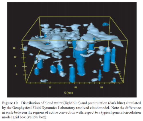
One of the big challenges in climate modeling (there are many) is model resolution and “sub-grid parameterization”. A climate model is created by breaking up the atmosphere (and ocean) into “small” cells of something like 200km x 200km, assigning one value in each cell for parameters like N-S wind, E-W wind and up-down wind – and solving the set of equations (momentum, heat transfer and so on) across the whole earth. However, in one cell like this below you have many small regions of rapidly ascending air (convection) topped by clouds of different thicknesses and different heights and large regions of slowly descending air:
Held and Soden (2000)
The model can’t resolve the actual processes inside the grid. That’s the nature of how finite element analysis works. So, of course, the “parameterization schemes” to figure out how much cloud, rain and humidity results from say a warming earth are problematic and very hard to verify.
Running higher resolution models helps to illuminate the subject. We can’t run these higher resolution models for the whole earth – instead all kinds of smaller scale model experiments are done which allow climate scientists to see which factors affect the results.
Here is the “plain language summary” from Organization of tropical convection in low vertical wind shears:Role of updraft entrainment, Tompkins & Semie 2017:
Thunderstorms dry out the atmosphere since they produce rainfall. However, their efficiency at drying the atmosphere depends on how they are arranged; take a set of thunderstorms and sprinkle them randomly over the tropics and the troposphere will remain quite moist, but take that same number of thunderstorms and place them all close together in a “cluster” and the atmosphere will be much drier.
Previous work has indicated that thunderstorms might start to cluster more as temperatures increase, thus drying the atmosphere and letting more infrared radiation escape to space as aresult – acting as a strong negative feedback on climate, the so-called iris effect.
We investigate the clustering mechanisms using 2km grid resolution simulations, which show that strong turbulent mixing of air between thunderstorms and their surrounding is crucial for organization to occur. However, with grid cells of 2 km this mixing is not modelled explicitly but instead represented by simple model approximations, which are hugely uncertain. We show three commonly used schemes differ by over an order of magnitude. Thus we recommend that further investigation into the climate iris feedback be conducted in a coordinated community model intercomparison effort to allow model uncertainty to be robustly accounted for.
And a little about computation resources and resolution. CRMs are “cloud resolving models”, i.e. higher resolution models over smaller areas:
In summary, cloud-resolving models with grid sizes of the order of 1 km have revealed many of the potential feed-back processes that may lead to, or enhance, convective organization. It should be recalled however, that these studies are often idealized and involve computational compromises, as recently discussed in Mapes [2016]. The computational requirements of RCE experiments that require more than 40 days of integration still largely prohibit horizontal resolutions finer than 1 km. Simulations such as Tompkins [2001c], Bryan et al. [2003], and Khairoutdinov et al. [2009] that use resolutions less than 350 m were restricted to 1 or 2 days. If water vapor entrainment is a factor for either the establishment and/or the amplification of convective organization, it raises the issue that the organization strength in CRMs model using grid sizes of the order of 1 km or larger is likely to be sensitive to the model resolution and simulation framework in terms of the choice of subgrid-scale diffusion and mixing.
In their conclusion on what resolution is needed:
.. and states that convergence is achieved when the most energetic eddies are well resolved, which is not the case at 2 km, and Craig and Dornbrack [2008] also suggest that resolving clouds requires grid sizes that resolve the typical buoyancy scale of a few hundred meters. The present state of the art of LES is represented by Heinze et al. [2016], integrating a model for the whole of Germany with a 100 m grid spacing, for a period of 4 days.
They continue:
The simulations in this paper also highlight the fact that intricacies of the assumptions contained in the parameterization of small- scale physics can strongly impact the possibility of crossing the threshold from unorganized to organized equilibrium states. The expense of such simulations has usually meant that only one model configuration is used concerning assumptions of small-scale processes such as mixing and microphysics, often initialized from a single initial condition. The potential of multiple equilibria and also an hysteresis in the transition between organized and unorganized states [Muller and Held, 2012], points to the requirement for larger integration ensembles employing a range of initial and boundary conditions, and physical parameterization assumptions. The ongoing requirements of large-domain, RCE numerical experiments imply that this challenge can be best met with a community-based, convective organization model intercomparison project (CORGMIP).
Here is Detailed Investigation of the Self-Aggregation of Convection in Cloud-Resolving Simulations, Muller & Held (2012). The second author is Isaac Held, often referenced on this blog who has been writing very interesting papers for about 40 years:
It is well known that convection can organize on a wide range of scales. Important examples of organized convection include squall lines, mesoscale convective systems (Emanuel 1994; Holton 2004), and the Madden– Julian oscillation (Grabowski and Moncrieff 2004). The ubiquity of convective organization above tropical oceans has been pointed out in several observational studies (Houze and Betts 1981; WCRP 1999; Nesbitt et al. 2000)..
..Recent studies using a three-dimensional cloud resolving model show that when the domain is sufficiently large, tropical convection can spontaneously aggregate into one single region, a phenomenon referred to as self-aggregation (Bretherton et al. 2005; Emanuel and Khairoutdinov 2010). The final climate is a spatially organized atmosphere composed of two distinct areas: a moist area with intense convection, and a dry area with strong radiative cooling (Figs. 1b and 2b,d). Whether or not a horizontally homogeneous convecting atmosphere in radiative convective equilibrium self-aggregates seems to depend on the domain size (Bretherton et al. 2005). More generally, the conditions under which this instability of the disorganized radiative convective equilibrium state of tropical convection occurs, as well as the feedback responsible, remain unclear.
We see the difference in self-aggregation of convection between the two domain sizes below:
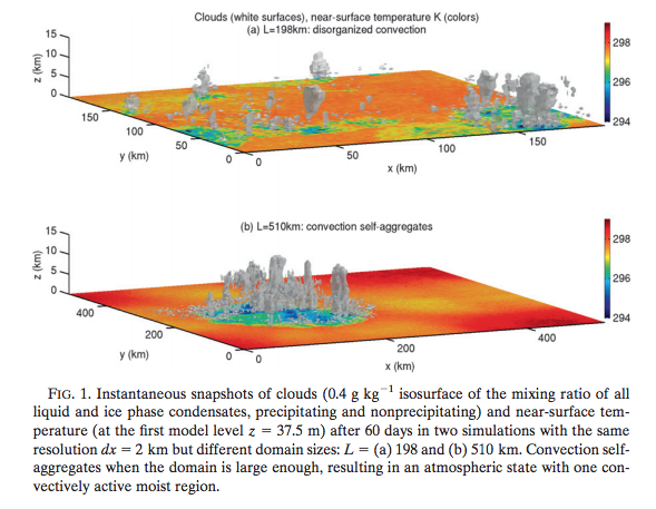
From Muller & Held 2012
Figure 1
The effect on rainfall and OLR (outgoing longwave radiation) is striking, and also note that the mean is affected:
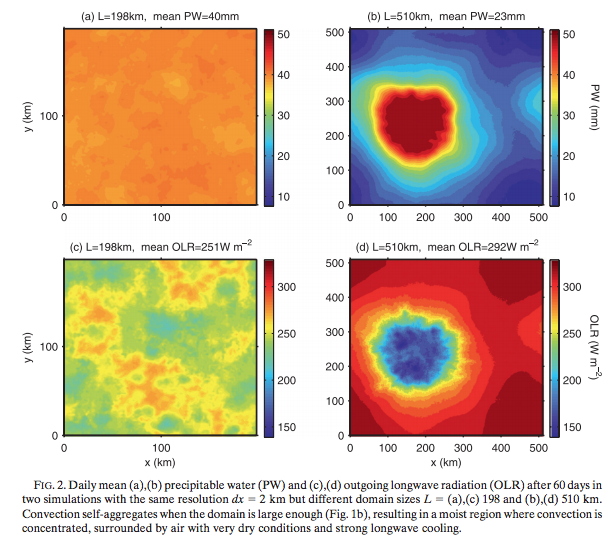
From Muller & Held 2012
Figure 2
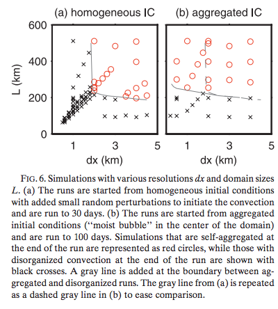
Then they look at varying model resolution (dx), domain size (L) and also the initial conditions. The higher resolution models don’t produce the self-aggregation, but the results are also sensitive to domain size and initial conditions. The black crosses denote model runs where the convection stayed disorganized, the red circles where the convection self-aggregated:
From Muller & Held 2012
Figure 3
In their conclusion:
The relevance of self-aggregation to observed convective organization (mesoscale convective systems, mesoscale convective complexes, etc.) requires further investigation. Based on its sensitivity to resolution (Fig. 6a), it may be tempting to see self-aggregation as a numerical artifact that occurs at coarse resolutions, whereby low-cloud radiative feedback organizes the convection.
Nevertheless, it is not clear that self-aggregation would not occur at fine resolution if the domain size were large enough. Furthermore, the hysteresis (Fig. 6b) increases the importance of the aggregated state, since it expands the parameter span over which the aggregated state exists as a stable climate equilibrium. The existence of the aggregated state appears to be less sensitive to resolution than the self-aggregation process. It is also possible that our results are sensitive to the value of the sea surface temperature; indeed, Emanuel and Khairoutdinov (2010) find that warmer sea surface temperatures tend to favor the spontaneous self-aggregation of convection.
Current convective parameterizations used in global climate models typically do not account for convective organization.
More two-dimensional and three dimensional simulations at high resolution are desirable to better understand self-aggregation, and convective organization in general, and its dependence on the subgrid-scale closure, boundary layer, ocean surface, and radiative scheme used. The ultimate goal is to help guide and improve current convective parameterizations.
From the results in their paper we might think that self-aggregation of convection was a model artifact that disappears with higher resolution models (they are careful not to really conclude this). Tompkins & Semie 2017 suggested that Muller & Held’s results may be just a dependence on their sub-grid parameterization scheme (see note 1).
From Hohenegger & Stevens 2016, how convection self-aggregates over time in their model:
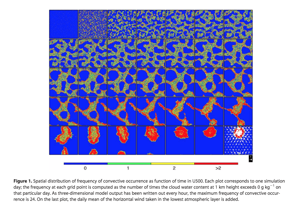
From Hohenegger & Stevens 2016
Figure 4 – Click to enlarge
From a review paper on the same topic by Wing et al 2017:
The novelty of self-aggregation is reflected by the many remaining unanswered questions about its character, causes and effects. It is clear that interactions between longwave radiation and water vapor and/or clouds are critical: non-rotating aggregation does not occur when they are omitted. Beyond this, the field is in play, with the relative roles of surface fluxes, rain evaporation, cloud versus water vapor interactions with radiation, wind shear, convective sensitivity to free atmosphere water vapor, and the effects of an interactive surface yet to be firmly characterized and understood.
The sensitivity of simulated aggregation not only to model physics but to the size and shape of the numerical domain and resolution remains a source of concern about whether we have even robustly characterized and simulated the phenomenon. While aggregation has been observed in models (e.g., global models) in which moist convection is parameterized, it is not yet clear whether such models simulate aggregation with any real fidelity. The ability to simulate self-aggregation using models with parameterized convection and clouds will no doubt become an important test of the quality of such schemes.
Understanding self-aggregation may hold the key to solving a number of obstinate problems in meteorology and climate. There is, for example, growing optimism that understanding the interplay among radiation, surface fluxes, clouds, and water vapor may lead to robust accounts of the Madden Julian oscillation and tropical cyclogenesis, two long-standing problems in atmospheric science.
Indeed, the difficulty of modeling these phenomena may be owing in part to the challenges of simulating them using representations of clouds and convection that were not designed or tested with self-aggregation in mind.
Perhaps most exciting is the prospect that understanding self-aggregation may lead to an improved understanding of climate. The strong hysteresis observed in many simulations of aggregation—once a cluster is formed it tends to be robust to changing environmental conditions—points to the possibility of intransitive or almost intransitive behavior of tropical climate.
The strong drying that accompanies aggregation, by cooling the system, may act as a kind of thermostat, if indeed the existence or degree of aggregation depends on temperature. Whether or how well this regulation is simulated in current climate models depends on how well such models can simulate aggregation, given the imperfections of their convection and cloud parameterizations.
Clearly, there is much exciting work to be done on aggregation of moist convection.
[Emphasis added]
Conclusion
Climate science asks difficult questions that are currently unanswerable. This goes against two myths that circulate media and many blogs: on the one hand the myth that the important points are all worked out; and on the other hand the myth that climate science is a political movement creating alarm, with each paper reaching more serious and certain conclusions than the paper before. Reading lots of papers I find a real science. What is reported in the media is unrelated to the state of the field.
At the heart of modeling climate is the need to model turbulent fluid flows (air and water) and this can’t be done. Well, it can be done, but using schemes that leave open the possibility or probability that further work will reveal them to be inadequate in a serious way. Running higher resolution models helps to answer some questions, but more often reveals yet new questions. If you have a mathematical background this is probably easy to grasp. If you don’t it might not make a whole lot of sense, but hopefully you can see from the papers that very recent papers are not yet able to resolve some challenging questions.
At some stage sufficiently high resolution models will be validated and possibly allow development of more realistic parameterization schemes for GCMs. For example, here is Large-eddy simulations over Germany using ICON: a comprehensive evaluation, Reike Heinze et al 2016, evaluating their model with 150m grid resolution – 3.3bn grid points on a sub-1 second time step over 4 days over Germany:
These results consistently show that the high-resolution model significantly improves the representation of small- to mesoscale variability. This generates confidence in the ability to simulate moist processes with fidelity. When using the model output to assess turbulent and moist processes and to evaluate and develop climate model parametrizations, it seems relevant to make use of the highest resolution, since the coarser-resolved model variants fail to reproduce aspects of the variability.
Related Articles
Ensemble Forecasting – why running a lot of models gets better results than one “best” model
Latent heat and Parameterization – example of one parameterization and its problems
Turbulence, Closure and Parameterization – explaining how the insoluble problem of turbulence gets handled in models
Part Four – Tuning & the Magic Behind the Scenes – how some important model choices get made
Part Five – More on Tuning & the Magic Behind the Scenes – parameterization choices, aerosol properties and the impact on temperature hindcasting, plus a high resolution model study
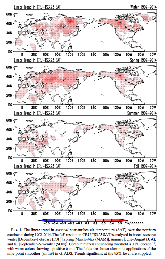
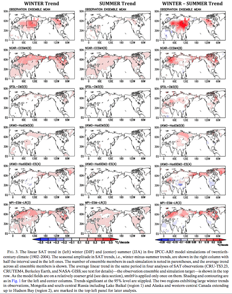
Part Six – Tuning and Seasonal Contrasts – model targets and model skill, plus reviewing seasonal temperature trends in observations and models
References
Missing iris efect as a possible cause of muted hydrological change and high climate sensitivity in models, Thorsten Mauritsen and Bjorn Stevens, Nature Geoscience (2015) – free paper
Organization of tropical convection in low vertical wind shears:Role of updraft entrainment, Adrian M Tompkins & Addisu G Semie, Journal of Advances in Modeling Earth Systems (2017) – free paper
Detailed Investigation of the Self-Aggregation of Convection in Cloud-Resolving Simulations, Caroline Muller & Isaac Held, Journal of the Atmospheric Sciences (2012) – free paper
Coupled radiative convective equilibrium simulations with explicit and parameterized convection, Cathy Hohenegger & Bjorn Stevens, Journal of Advances in Modeling Earth Systems (2016) – free paper
Convective Self-Aggregation in Numerical Simulations: A Review, Allison A Wing, Kerry Emanuel, Christopher E Holloway & Caroline Muller, Surv Geophys (2017) – free paper
Large-eddy simulations over Germany using ICON: a comprehensive evaluation, Reike Heinze et al, Quarterly Journal of the Royal Meteorological Society (2016)
Other papers worth reading:
Featured Article Self-aggregation of convection in long channel geometry, Allison A Wing & Timothy W Cronin, Quarterly Journal of the Royal Meteorological Society (2016) – paywall paper
Notes
Note 1: The equations for turbulent fluid flow are insoluble due to the computing resources required. Energy gets dissipated at the scales where viscosity comes into play. In air this is a few mm. So even much higher resolution models like the cloud resolving models (CRMs) with scales of 1km or even smaller still need some kind of parameterizations to work. For more on this see Turbulence, Closure and Parameterization.