I’ve had questions about the use of ensembles of climate models for a while. I was helped by working through a bunch of papers which explain the origin of ensemble forecasting. I still have my questions but maybe this post will help to create some perspective.
The Stochastic Sixties
Lorenz encapulated the problem in the mid-1960’s like this:
The proposed procedure chooses a finite ensemble of initial states, rather than the single observed initial state. Each state within the ensemble resembles the observed state closely enough so that the difference might be ascribed to errors or inadequacies in observation. A system of dynamic equations previously deemed to be suitable for forecasting is then applied to each member of the ensemble, leading to an ensemble of states at any future time. From an ensemble of future states, the probability of occurrence of any event, or such statistics as the ensemble mean and ensemble standard deviation of any quantity, may be evaluated.
Between the near future, when all states within an ensemble will look about alike, and the very distant future, when two states within an ensemble will show no more resemblance than two atmospheric states chosen at random, it is hoped that there will be an extended range when most of the states in an ensemble, while not constituting good pin-point forecasts, will possess certain important features in common. It is for this extended range that the procedure may prove useful.
[Emphasis added].
Epstein picked up some of these ideas in two papers in 1969. Here’s an extract from The Role of Initial Uncertainties in Prediction.
While it has long been recognized that the initial atmospheric conditions upon which meteorological forecasts are based are subject to considerable error, little if any explicit use of this fact has been made.
Operational forecasting consists of applying deterministic hydrodynamic equations to a single “best” initial condition and producing a single forecast value for each parameter..
..One of the questions which has been entirely ignored by the forecasters.. is whether of not one gets the “best” forecast by applying the deterministic equations to the “best” values of the initial conditions and relevant parameters..
..one cannot know a uniquely valid starting point for each forecast. There is instead an ensemble of possible starting points, but the identification of the one and only one of these which represents the “true” atmosphere is not possible.
In essence, the realization that small errors can grow in a non-linear system like weather and climate leads us to ask what the best method is of forecasting the future. In this paper Epstein takes a look at a few interesting simple problems to illustrate the ensemble approach.
Let’s take a look at one very simple example – the slowing of a body due to friction.
Rate of change of velocity (dv/dt) is proportional to the velocity, v. The “proportional” term is k, which increases with more friction.
dv/dt = -kv, therefore, v = v0.exp(-kt), where v0 = initial velocity
With a starting velocity of 10 m/s and k = 10-4 (in units of 1/s), how does velocity change with time?

Figure 1 – note the logarithm of time on the time axis, time runs from 10 secs – 100,000 secs
Probably no surprises there.
Now let’s consider in the real world that we don’t know the starting velocity precisely, and also we don’t know the coefficient of friction precisely. Instead, we might have some idea about the possible values, which could be expressed as a statistical spread. Epstein looks at the case for v0 with a normal distribution and k with a gamma distribution (for specific reasons not that important).
Mean of v0: <v0> = 10 m/s
Standard deviation of v0: σv = 1m/s
Mean of k: <k> = 10-4 /s
Standard deviation of k: σk = 3×10⁻⁵ /s
The particular example he gave has equations that can be easily manipulated, allowing him to derive an analytical result. In 1969 that was necessary. Now we have computers and some lucky people have Matlab. My approach uses Matlab.
What I did was create a set of 1,000 random normally distributed values for v0, with the mean and standard deviation above. Likewise, a set of gamma distributed values for k.
Then we take each pair in turn and produce the velocity vs time curve. Then we look at the stats of the 1,000 curves.
Interestingly the standard deviation increases before fading away to zero. It’s easy to see why the standard deviation will end up at zero – because the final velocity is zero. So we could easily predict that. But it’s unlikely we would have predicted that the standard deviation of velocity would start to increase after 3,000 seconds and then peak at around 9,000 seconds.
Here is the graph of standard deviation of velocity vs time:
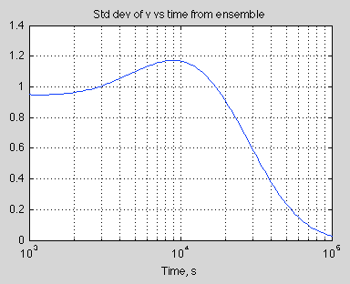
Figure 2
Now let’s look at the spread of results. The blue curves in the top graph (below) are each individual ensemble member and the green is the mean of the ensemble results. The red curve is the calculation of velocity against time using the mean of v0 and k:
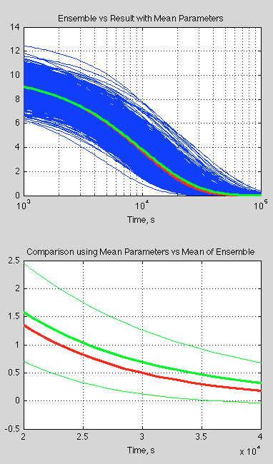
Figure 3
The bottom curve zooms in on one portion (note the time axis is now linear), with the thin green lines being 1 standard deviation in each direction.
What is interesting is the significant difference between the mean of the ensemble members and the single value calculated using the mean parameters. This is quite usual with “non-linear” equations (aka the real world).
So, if you aren’t sure about your parameters or your initial conditions, taking the “best value” and running the simulation can well give you a completely different result from sampling the parameters and initial conditions and taking the mean of this “ensemble” of results..
Epstein concludes in his paper:
In general, the ensemble mean value of a variable will follow a different course than that of any single member of the ensemble. For this reason it is clearly not an optimum procedure to forecast the atmosphere by applying deterministic hydrodynamic equations to any single initial condition, no matter how well it fits the available, but nevertheless finite and fallible, set of observations.
In Epstein’s other 1969 paper, Stochastic Dynamic Prediction, is more involved. He uses Lorenz’s “minimum set of atmospheric equations” and compares the results after 3 days from using the “best value” starting point vs an ensemble approach. The best value approach has significant problems compared with the ensemble approach:
Note that this does not mean the deterministic forecast is wrong, only that it is a poor forecast. It is possible that the deterministic solution would be verified in a given situation but the stochastic solutions would have better average verification scores.
Parameterizations
One of the important points in the earlier work on numerical weather forecasting was the understanding that parameterizations also have uncertainty associated with them.
For readers who haven’t seen them, here’s an example of a parameterization, for latent heat flux, LH:
LH = LρCDEUr(qs-qa)
which says Latent Heat flux = latent heat of vaporization x density x “aerodynamic transfer coefficient” x wind speed at the reference level x ( humidity at the surface – humidity in the air at the reference level)
The “aerodynamic transfer coefficient” is somewhere around 0.001 over ocean to 0.004 over moderately rough land.
The real formula for latent heat transfer is much simpler:
LH = the covariance of upwards moisture with vertical eddy velocity x density x latent heat of vaporization
These are values that vary even across very small areas and across many timescales. Across one “grid cell” of a numerical model we can’t use the “real formula” because we only get to put in one value for upwards eddy velocity and one value for upwards moisture flux and anyway we have no way of knowing the values “sub-grid”, i.e., at the scale we would need to know them to do an accurate calculation.
That’s why we need parameterizations. By the way, I don’t know whether this is a current formula in use in NWP, but it’s typical of what we find in standard textbooks.
So right away it should be clear why we need to apply the same approach of ensembles to the parameters describing these sub-grid processes as well as to initial conditions. Are we sure that over Connecticut the parameter CDE = 0.004, or should it be 0.0035? In fact, parameters like this are usually calculated from the average of a number of experiments. They conceal as much as they reveal. The correct value probably depends on other parameters. In so far as it represents a real physical property it will vary depending on the time of day, seasons and other factors. It might even be, “on average”, wrong. Because “on average” over the set of experiments was an imperfect sample. And “on average” over all climate conditions is a different sample.
The Numerical Naughties
The insights gained in the stochastic sixties weren’t so practically useful until some major computing power came along in the 90s and especially the 2000s.
Here is Palmer et al (2005):
Ensemble prediction provides a means of forecasting uncertainty in weather and climate prediction. The scientific basis for ensemble forecasting is that in a non-linear system, which the climate system surely is, the finite-time growth of initial error is dependent on the initial state. For example, Figure 2 shows the flow-dependent growth of initial uncertainty associated with three different initial states of the Lorenz (1963) model. Hence, in Figure 2a uncertainties grow significantly more slowly than average (where local Lyapunov exponents are negative), and in Figure 2c uncertainties grow significantly more rapidly than one would expect on average. Conversely, estimates of forecast uncertainty based on some sort of climatological-average error would be unduly pessimistic in Figure 2a and unduly optimistic in Figure 2c.
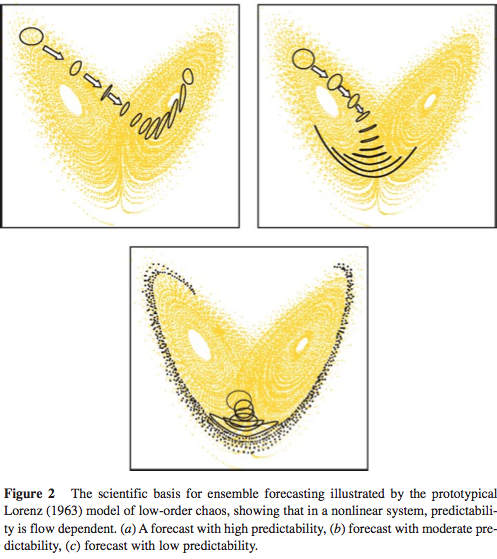
From Palmer et al 2005
Figure 4
The authors then provide an interesting example to demonstrate the practical use of ensemble forecasts. In the top left are the “deterministic predictions” using the “best estimate” of initial conditions. The rest of the charts 1-50 are the ensemble forecast members each calculated from different initial conditions. We can see that there was a low yet significant chance of a severe storm:
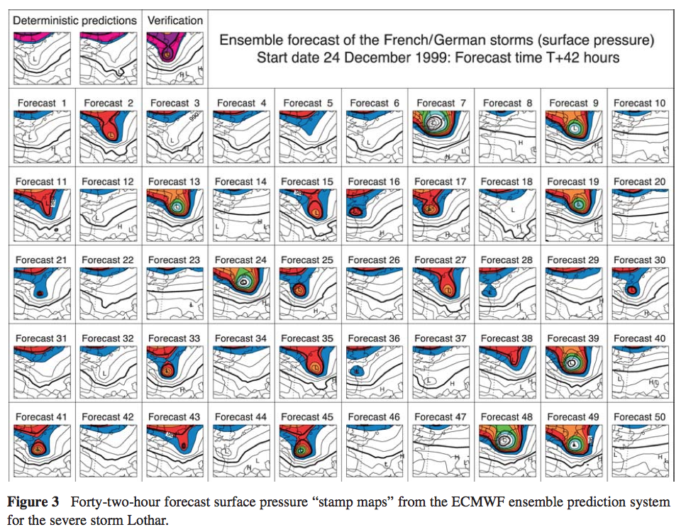
From Palmer et al 2005
Figure 5 – Click to enlarge
In fact a severe storm did occur so the probabilistic forecast was very useful, in that it provided information not available with the deterministic forecast.
This is a nice illustration of some benefits. It doesn’t tell us how well NWPs perform in general.
One measure is the forecast spread of certain variables as the forecast time increases. Generally single model ensembles don’t do so well – they under-predict the spread of results at later time periods.
Here’s an example of the performance of a multi-model ensemble vs single-model ensembles on saying whether an event will occur or not. (Intuitively, the axes seem the wrong way round). The single model versions are over-confident – so when the forecast probability is 1.0 (certain) the reality is 0.7; when the forecast probability is 0.8, the reality is 0.6; and so on:
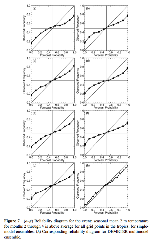
From Palmer et al 2005
Figure 6
We can see that, at least in this case, the multi-model did a pretty good job. However, similar work on forecasting precipitation events showed much less success.
In their paper, Palmer and his colleagues contrast multi-model vs multi-parameterization within one model. I am not clear what the difference is – whether it is a technicality or something fundamentally different in approach. The example above is multi-model. They do give some examples of multi-parameterizations (with a similar explanation to what I gave in the section above). Their paper is well worth a read, as is the paper by Lewis (see links below).
Discussion
The concept of taking a “set of possible initial conditions” for weather forecasting makes a lot of sense. The concept of taking a “set of possible parameterizations” also makes sense although it might be less obvious at first sight.
In the first case we know that we don’t know the precise starting point because observations have errors and we lack a perfect observation system. In the second case we understand that a parameterization is some empirical formula which is clearly not “the truth”, but some approximation that is the best we have for the forecasting job at hand, and the “grid size” we are working to. So in both cases creating an ensemble around “the truth” has some clear theoretical basis.
Now what is also important for this theoretical basis is that we can test the results – at least with weather prediction (NWP). That’s because of the short time periods under consideration.
A statement from Palmer (1999) will resonate in the hearts of many readers:
A desirable if not necessary characteristic of any physical model is an ability to make falsifiable predictions
When we come to ensembles of climate models the theoretical case for multi-model ensembles is less clear (to me). There’s a discussion in IPCC AR5 that I have read. I will follow up the references and perhaps produce another article.
References
The Role of Initial Uncertainties in Prediction, Edward Epstein, Journal of Applied Meteorology (1969) – free paper
Stochastic Dynamic Prediction, Edward Epstein, Tellus (1969) – free paper
On the possible reasons for long-period fluctuations of the general circulation. Proc. WMO-IUGG Symp. on Research and Development Aspects of Long-Range Forecasting, Boulder, CO, World Meteorological Organization, WMO Tech. EN Lorenz (1965) – cited from Lewis (2005)
Roots of Ensemble Forecasting, John Lewis, Monthly Weather Forecasting (2005) – free paper
Predicting uncertainty in forecasts of weather and climate, T.N. Palmer (1999), also published as ECMWF Technical Memorandum No. 294 – free paper
Representing Model Uncertainty in Weather and Climate Prediction, TN Palmer, GJ Shutts, R Hagedorn, FJ Doblas-Reyes, T Jung & M Leutbecher, Annual Review Earth Planetary Sciences (2005) – free paper


Ensemble forecasts seem to be making their way towards public availability. I have no idea about their general availability in different countries, but here in Finland both locally operating services make them available:
http://en.ilmatieteenlaitos.fi/weather/espoo?forecast=long
http://www.foreca.se/Finland/S%C3%B6dra-Finland/Esbo/15-dygnsprognos
In the case of Foreca only the pages in Finnish and Swedish show the ensemble forecasts. (I linked the latter as it may be a little easier to understand:)
If I understand correctly, the typical charts for temperature projections are based on multi-model ensemble forecasts. And the resulting projection is typically the average of the projections, and the resulting error bars represent the variability of that average.
This may give a rather different result from including the variability of all the projections in the ensemble, underestimating the true range of a given projection scenario. IOW, it’s going to make our forecasts look a lot more certain than they really are.
I recognize that there are legitimate difficulties in getting a truer uncertainty range, particularly in figuring out how to weight different models. Still, I expect that it will be better to take a best guess on weighting models than to present a deceptive picture of overcertain forecasts. It reminds me of the hockey stick “trick” – what is being calculated and shown is actually quite well-documented, but those people who don’t dig deeply into the problem are going to get the wrong impression, and that has the potential to hurt the debate.
If the actual observed surface temperatures go outside the ensemble forecast range, then one might get an incorrect impression that the models are “wrong”, simply based on a bad calculation of the “uncertainty”.
Or am I just way off base here? I might misunderstand how the ensemble forecast uncertainties are calculated.
Windchasers,
I don’t really understand the climate model ensembles.
NWP (numerical weather prediction) is a bit clearer in my mind. For different initial conditions we can simply look at the stats of the results. So long as we are choosing the initial conditions for the ensemble from a representative sample. When it comes to ensembles of parameters in NWP I believe it’s the same approach.
For climate models I have lots of questions. They are based on the same physics as NWP, although larger grid size and larger time steps – therefore more parameterizations – but fundamentally the same sets of equations.
More on this later.
Some of the questions in my mind about climate models..
If weather is an “initial value problem” and climate is not (as many people say) then why do we need ensembles of the same model?
If climate is an initial value problem then it’s a different story.
The role of a climate model (see note 1) is to provide future states of weather (under different scenarios) that we can aggregate into statistics we call climate. In this way we hope to predict the future state of the climate.
Different model runs of the same model with the same parameters apparently produce different statistics. Why? Is this just because one run provides incomplete information, i.e., we don’t have enough sample data from the last 20 years of one run to predict “climate”. In that case, is this the same as sampling over more time (obviously there would be a problem doing this to forecast for transient conditions)?
So if we wanted to predict the equilibrium climate after say CO2 had doubled, is 10 runs of 100 years the same as 1 run of 1000 years? If so, has this been verified?
Another question relates to multi-model ensembles. I see the case (as laid out in the article) for ensembles of initial conditions and ensembles of parameters for weather forecasting. It’s not a big stretch to see multi-model ensembles (for weather forecasting) as simply another approach to multi-parameter ensembles.
This has a theoretical justification. And of course we can test and refine pretty quickly with NWP.
With climate models what is the mean and standard deviation of different model runs actually producing?
Suppose:
Climate model A has a persistent cold bias in the northern polar regions but gets overall rainfall distribution pretty good.
Climate model B has no strong temperature bias but has a bad rainfall distribution in the tropics.
It’s pretty clear that averaging model A and model B will produce overall better climate statistics – the result looks better.
This is my working theory (hopefully someone will prove me wrong) on why ensembles of different climate models have been used.
A different approach would be to say that although the result looks better it isn’t actually valid to just average models that produce fundamentally different and flawed climates (note 2). Is averaging two flaws the right answer? (Obviously lots of people work on investigating flaws and thus improving the representation of climate in models).
Lots of questions..
Note 1 – Climate models have many other uses: one example is to help us understand the interactions between different aspects of the climate and test hypotheses. In the case above I am referring to the role of the climate model in helping us see what the future will look like with more GHGs.
Note 2 – Of course, we could now take this to a ridiculous point where ensembles are never allowed if any one of 20 parameters across any point on the globe was out by 0.1%. That’s not what I’m trying to suggest.
SoD,
Some of your questions can be answered by noting that GCMs developed for climate research are not really directly climate models, they are crude weather models. An ensemble calculation by such a model may be considered “a climate model”, i.e. a model based process that produces as outcome climate indicators like average temperatures and other statistical indicators.
I have read somewhere that that very long model runs have been used as an alternative for many separate runs with different initial values. As far as I have understood the results have been essentially the same. As you write, this is possible only for stationary conditions.
The spaghetti graphs presented in IPCC reports tell directly, how ensembles have been used in climate research.
Pekka,
I believe that’s correct. They spin up the model until it’s stable and then run it for, say, 100 years. Then they chose different times in those 100 years as the initial conditions to start changing inputs like CO2. However, I’m not at all sure that the results of using different starting points produces results with negligible differences. That may well be model dependent.
Three points, preliminaries before I can respond with a result based upon thinking about this excellent post and its comments for a while.
First, climate models as currently practiced are practical computational beasts in that they get as much as they can out of the computer hardware they run upon. These hardware systems as massive — but not anywhere as massive as could be applied (and that, in my opinion, is tragic) — yet use grid cells on the order of tens of kilometers. Also, they use calibrated approximations in many of their parts, not because better models aren’t known, but because of the sheer need for computational speed. With all that, they are capable of great accuracy and precision. No doubt, they could be improved. There are concrete proposals for how they could be improved. Alas, at least this year, the U.S. Congress chose not to improve them.
Second, there are important limitations of what these models can include. Ice sheet dynamics, even as understood they are, which is poor, are not included at all. They should be, and we should know more about these.
Third, there are, as I believe, basic problems with ensemble models as described. First, these are deterministic models, and some people feel, they should be stochastic ones. That is, the basic interior of these models should be probabilistic calculations, and present day models are not … They tend to use expected, single point values and project these. If at any point any of the distributions of these random variables are multimodal, these could be severely misleading. There are proposals for changing models in this way, or at least experimenting with these variants. Alas, these have not been funded, as yet, at least not in the United States.
There’s a basic question about how Earth’s climate works. It’s my personal technical opinion that each step of state evolution Earth’s climate takes is fundamentally stochastic, so two runs of even the actual climate from the same starting point will land in a different place, even if the starting point could be identified to infinite precision (which, of course, it cannot be). I’ve been reminded in my studies of these systems that Navier-Stokes is an approximation, even as complicated as it is.
“Navier-Stokes is an approximation” ?
You mean any solutions are approximations? The equations themselves are first principles derivations. Did I miss something?
Navier-Stokes equation is a continuum equation, but no real fluid is a continuum, but formed from molecules. There are open fundamental questions on the mathematical properties of N-S equation: Do they really posses any solutions?
I’m not at all certain of the following, but my impression is that some of the most important open questions about N-S equation are related to the continuum approximation to the non-continuum real world. In other words, some of the fundamental problems of real non-continuum fluid mechanics are not the same as those of N-S equation.
Pekka,
The same could be said about most equations in physics.
The N-S equations are derived from conservation of momentum and conservation of mass. The problem of these equations is how to solve them in practice. This doesn’t involve the fact that there are 10x molecules per m3.
Here’s a quote from Durbin & Reif, Statistical Theory and Modeling for Turbulent Flows, (2010):
SoD,
Equations of the general type of N-S may lead to problems at very short distances or at very large distances. In many cases it’s relatively easy to prove that no such problems are present, while there are other cases, where the problems are serious. The infrared and ultraviolet catastrophes of various theories are strong examples of that.
The problems of the Navier-Stokes equations are perhaps not as dramatic, but significant enough to make it one of the Millenium Prize Problems of the Clay Mathematics Institute
http://www.claymath.org/millenium-problems/navier%E2%80%93stokes-equation
I don’t know details of fluid mechanics well, but am learning some in conjunction with studies of physical oceanography, principally using texts by Knauss (Introduction to Physical Oceanography), and Pond and Pickard (Introductory Dynamical Oceanography, 2nd edition). I also have, as a reference, Kundu and Cohen (Fluid Mechanics, 3rd edition). There is also a small section on geophysical fluid mechanics at the back of Ray Pierrehumbert’s Principles of Planetary Climate.
I recently came across a direct mention of the inadequacy of Navier-Stokes some place, with the suggestion that in some cases only full Newtonian simulation of molecules might capture phenomena. That’s an audacious claim, I know, but unfortunately I don’t recall where I read it.
However, there are two explanations in two of the cited references for why Navier-Stokes is wanting, at least in oceanic problems.
One, from Pond and Pickard, is the need to include frictional terms in the equations for high Reynolds Number turbulent oceanic flows which, paraphrasing their presentation (page 50, section 7.20), involve a Taylor expansion about mean flow. The attempt to “close” the equations in section 7.21 involves the introduction of a notion eddy viscosity which, as is highlighted, is a property not of the fluid but of the flow itself, something which is inherently difficult to observe and, so, calibrate.
The other, from Kundu and Cohen, in their treatment of incompressible viscous fluid flow, pertains to “Convection-Dominated Problems” (Chapter 11 on Computational Fluid Dynamics, authored by Hu, pages 402-403). The text points out that “unphysical oscillations” can develop in computational solutions at boundary layers when the grid is not sufficiently fine to resolve the rapid variation of the computational solution. Variable grid sizing in proposed as a means of resolving the flow, something I know is done in, e.g., WHOI’s FVCOM system. Kundu and Cohen’s Hu explains that the grid size is made small enough so the Peclet Number within the cell is smaller than two. The Peclet Number is the product of the Reynolds Number and the viscous diffusion rate divided by the mass or molecular diffusion rate.
I don’t know much about the innards of climate models like CMIP5 to say what they do in these regards. I know FVCOM is pretty special (and computationally intensive) as it can resolve near coastal wave turbulence, e.g., the tsunami waves which disrupted northeast Japan in 2011 (see also this movie, and this article).
Whether the Navier-Stokes equation is accurate and solvable in principle, it’s definitely not presently possible to describe turbulence based directly on N-S equation in any demanding application. To get reasonable results for turbulent flow in practical applications one of several alternative approximate descriptions (or parameterizations) of turbulent flow must be chosen and applied. Many well known models are listed here
http://www.cfd-online.com/Wiki/Turbulence_modeling
There’s also some discussion of direct numerical simulation and its inadequacy in that link.
Atmosphere has eddies both at subgrid-scale and at a significantly larger scale. The models can describe the largest scales at least qualitatively, but the influence of subgrid-scale phenomena must be included trough parameterization. I would expect that the situation is even worse with the eddies of oceans.
hypergeometric,
I think the examples you gave are about the problem of solving the equations in practice (rather than a limitation of the NS equations themselves).
The first example is one approach to solving averaged flows. “Closing the equations” relates to the problem that once you rewrite the equations to produce some statistical value you end up with an extra term (e.g., <x><y> ≠ <xy> so now you have one more variable, <xy>, but no more equations).
One solution – that is not practical – is to solve the NS equations completely for the chaotic flow field and then calculate the statistics. So the alternative solution – used in practice – is to find some additional “rules”, i.e., additional equations that can be used to close the set of equations.
Eddy diffusivity & eddy viscosity are “invented values” used in ocean circulation calculations. Viscosity is a fluid property that can be reliably measured. “Eddy viscosity” is a “parameter” relating to the flow in question. People try to find some rules to put boundaries on these averaged values, or do experimental work to determine what they are in practice for some particular cases.
So in ocean circulation calculations it is very common to see “vertical eddy diffusivity” with a large range (factor of 10 or 100) about its presumed values. Vertical eddy diffusivity doesn’t really exist, but it’s a necessary parameter to try and find some values for vertical flow.
The second example is a problem of trying to solve the NS equations numerically.
Climate models conserve heat, momentum & mass and use parameterizations (like vertical eddy diffusivity) to work out where everything goes and how fast. Actually until a decade ago they didn’t really conserve heat and momentum, they “topped up” the models with invented values (flux corrections) to keep everything from drifting into unphysical results, but that’s another story..
All that said, I’m a bit of a novice with fluid dynamics and trying to understand the subject better myself.
Thanks! Useful!
– Jan
Just a note for anyone wanting to use < and > in comments (as I just remembered when nothing showed up in a previous comment).
They don’t work if you use the keyboard value. WordPress thinks they are html tags.
You need to enter – without the spaces:
& lt ;
this will give you <
& gt;
this will give you >
SoD,
Nitpick.
Eddy diffusivity isn’t about mass flow exactly, it’s about mixing. Bomb 14C, heat and spikes of tracer compounds like sulfur hexafluoride transport much faster in the ocean than would be possible by classical diffusion. Eddy diffusivity is why it only takes a few strokes of a spoon in a cup to thoroughly mix milk with your tea or cream with your coffee. It’s turbulence over a large range of scale. Large scale motion is necessary for eddy diffusion to occur because, like all turbulence, eddy diffusion is an energy dissipative process that requires an energy input to continue. As a result, you can talk about things like turbulent kinetic energy.
I made a search with words “turbulent mixing”. That brought up this review article of Paul Dimotakis. The article contains some brief comments on mixing in the atmosphere and oceans:
SOD wrote: “By the way, I don’t know whether this is a current formula in use in NWP, but it’s typical of what we find in standard textbooks.” If you are interested, Isaac Held recently discussed how climate models calculate evaporation from the ocean at the link below.
http://www.gfdl.noaa.gov/blog/isaac-held/2014/06/26/47-relative-humidity-over-the-oceans/
Good point, I think I linked to that from an earlier thread..
The formula Isaac Held quotes is the same “bulk” method.
Weather models have a smaller grid size but I don’t believe there is any “inbetween formula” between the first principles method (covariance of eddy velocity and humidity) and the bulk formula.
SOD wrote: “The concept of taking a “set of possible initial conditions” for weather forecasting makes a lot of sense. The concept of taking a “set of possible parameterizations” also makes sense although it might be less obvious at first sight… When we come to ensembles of climate models the theoretical case for multi-model ensembles is less clear (to me).”
If you assume that different climate models are simply implementing the same physics with a different set of parameters, then a multi-model ensemble could be considered to be your “set of possible parameterizations”. If all models relied on an “aerodynamic transfer coefficient” and their parameter optimization process had led to slightly different values for this parameter, then the multi-model ensemble is exploring “parameter-space”. Unfortunately, parameter space is not being systematically explored.
Section 10.1 of AR4 WG1 says:
Many of the figures in Chapter 10 are based on the mean and spread of the multi-model ensemble of comprehensive AOGCMs. The reason to focus on the multi-model mean is that averages across structurally different models empirically show better large-scale agreement with observations, because individual model biases tend to cancel (see Chapter 8). The expanded use of multi-model ensembles of projections of future climate change therefore provides higher quality and more quantitative climate change information compared to the TAR. Even though the ability to simulate present-day mean climate and variability, as well as observed trends, differs across models, no weighting of individual models is applied in calculating the mean. Since the ensemble is strictly an ‘ensemble of opportunity’, without sampling protocol, the spread of models does not necessarily span the full possible range of uncertainty, and a statistical interpretation of the model spread is therefore problematic. However, attempts are made to quantify uncertainty throughout the chapter based on various other lines of evidence, including perturbed physics ensembles specifically designed to study uncertainty within one model framework, and Bayesian methods using observational constraints.
The phrases “an ensemble of opportunity” and “a statistical interpretation of the model spread is therefore problematic” are telling.
Frank,
AR5 (chapter 9) has some development over AR4. Not sure whether it is substantial. Section 9.2.2 (p754-755) looks at the ensemble questions and provides references.
Thanks for the reference. I hadn’t caught up on this subject. The phrase “ensemble of opportunity” came from at least one paper on the literature on this subject. IMO, the worst aspect of the WG1 reports are that they make statistical interpretations of the multi-model spread in many places (without caveats), even though they recognize that these interpretations are misleading at best and wrong at worst.
Regarding “multimodel spreads”, there’s no real reason to have those, if Bayesian averaging is used. I don’t know the methods used by IPCC well. But I know there’s a sense that they need statistical help, and there certainly are papers out there which have talk about this, e.g., results of this search.
But, practically speaking, policymakers have a hard time with anything other than point estimates. A Bayesian posterior is multimodal in general, e.g., the standard equilibrium climate sensitivity for CO2 doubling. These can be reduced to a point estimate, but that entails positing a loss function, and these depend upon who you ask. As statistician John Cook once remarked to me, these have “shed problems”: Everyone agrees that a shed should be built, but nearly everyone disagrees with one another on how it should look.
I don’t think they have changed anything important about ensembles of models between AR4 and AR5, just eliminated some of the candor. The IPCC’s “ensemble of opportunity” can’t represent the full range of possible future climates that are compatible with our understanding of physics.
In your Figure 3 above, you’ve incorporated the full range of uncertainty in k and v0 into your model. You are entitled to report that v(t=30,000) is projected to be 0.67 (0.15-1.30, 68% ci). Since the IPCC hasn’t systematically explored parameter uncertainty, they aren’t entitled (IMO) to say the temperature in 2100 is “likely” to be X-Y degK (70% ci) warmer than today under a particular scenario. AR4 makes this clearer than AR5.
(Your elegant examples make these concepts so easy to discuss.)
hypergeometric wrote: “Regarding “multimodel spreads”, there’s no real reason to have those, if Bayesian averaging is used. I don’t know the methods used by IPCC well.”
The IPCC combines a few to a dozen runs from more than a dozen models into one figure or confidence interval. Each run uses different initialization conditions, so the uncertainty that arises from initialization of a chaotic system is adequately represented in the output.
The same thing is not true for “parameter uncertainty”, and the IPCCs models contains dozens of adjustable parameters. SOD discusses above how a typical parameter used in a model – an “aerodynamic transfer coefficient” of about 0.001 over ocean to 0.004 over moderately rough land – can be used to model the transfer of latent heat from a large grid cell on the surface to a large grid cell in the atmosphere – even though this parameter is an average for convection that is highly variable on smaller scales. Let’s suppose that the parameter for oceans is expected to lie between 0.0005 and 0.0015 (with 95% confidence) based on laboratory experiments or a fine scale model using what SOD calls “real physics”. In the process of tuning a climate model, the aerodynamic transfer coefficient is adjusted to give the best match to a related observable like precipitation or albedo. Other parameters are tuned one at a time in the same manner. The order of parameter tuning influences the outcome of the tuning process because the parameters interact in surprising ways. It might turn out that all of the IPCC’s models chose an optimized “aerodynamic transfer coefficient” between 0.0011 and 0.0013. However, studies with large ensembles of simplified models (perturbed physics ensembles), which select their parameters by chance from within an appropriate range have shown that reasonable models of current climate can be made with an aerodynamic transfer coefficient anywhere between 0.0005 and 0.0015. The TCR of such ensembles varies over a wide range than the IPCCs models. The range of future climates for 2X or 3X CO2 compatible with known physics appears to be much wider than the range of climate model output used by the IPCC.
hypergeometric also wrote: “But, practically speaking, policymakers have a hard time with anything other than point estimates.” I think you are underestimating our politicians, who have useful experiences from polling and gambling. They may not have much experience with a 90% confidence interval, but they probably understand the probability of their opponent not rolling doubles in backgammon – equivalent to an 83% confidence interval. Our politicians may prefer to hear a simple point estimate for political reasons from their preferred expert, but those experts – if they are scientists – should provide a most likely value and an confidence interval.
Excellent explanation. Thanks!
It’s typical to say that the upper limit for weather forecasting period is about two weeks, and that beyond that the nature of possible forecasts changes as chaotic phenomena make regular type weather forecasts worthless. In ensemble forecasts that fact manifests as a spread of weather projections that’s nearly as wide as deduced from historical variability for that time of the year (and possibly even wider, if the historical variability is not used explicitly or implicitly as a constraint).
A potential problem with ensemble projections of climate is that the relevant time scale of chaos may be very long. Peter Stone has written some articles that seem interesting (although I don’t know, how well they describe best present understanding). In the 2004 paper Climate Prediction: The Limits of Ocean Models he writes:
In the text he refers also to the weak dissipation in the oceans. When the real dissipation is very weak it’s possible that problems of numerical approximation (numerical diffusion as one important example) may affect the outcome strongly. It’s also possible that all present models suffer from some common problems making the whole ensemble misplaced.
He presents some results from the few calculations that had already studied these issues. They confirm the extent of the problems as it was seen in 2004.
Pekka,
Very interesting paper. I have a couple of Peter Stone’s early papers from the late 70s:
– Atmospheric Lapse Rate Regimes and Their Parameterization
– Baroclinic Adjustment
He makes some excellent points in this paper – points that I want to pick up and develop in the next series: Natural Variability and Chaos.
A good reference on turbulent flows is the text book “A First Course in Turbulence” by Tennekes and Lumley. Interestingly, H. Tennekes, was dismissed from his work position due to his being a skeptic on the global warming issue.
The problem with models is not just that complex turbulent flows cannot be exactly solved by Navier Stokes equations due to the fact that there are always more unknowns than equations, there is also the fact that much more of the physics of the Earths atmosphere/biosphere/oceans/surface and the Sun are not fully understood. Long period ocean currents, solar UV variation, cloud interactions, and aerosols variation are only a few of the poorly known terms. Approximating these effects and using unsolvable maths means that the problem is more than just an exactly defined but chaotic problem with limited accuracy on initial and boundary condition, it is a poorly posed problem, and even using a short history of data to approximate inputting unknown terms would surely fail as a general predictor of future outcomes. In other words, climate is as poorly predictable as weather.
This does not mean that an effort to estimate an effect of adding CO2, with no other change, and assuming no natural variation shift, should not be made, to see if it could be a problem. It just means look at real data and be honest that any effect might be less than expected, and lack of all important understanding truly limits what should be claimed.
The scare tactics gained a lot of funding for many researchers, so they tended to ignore the skeptics, who threatened their funding. This issue has resulted in a sad day for science.
Um, well surely whatever the dissipative mechanism for energy within oceans and atmosphere, it would be quite a finding if it were shown that could account for radiative forcing at 1+ Watts per square meter. That would mean that turbulence and mixing offsets overall planetary physics. It would be as if Newton’s laws could not be used to approximately predict a ball’s trajectory flying through air due to atmospheric drag and friction.
Now, undoubtedly if the fluid is viscous enough, Newton’s laws are not going to be helpful to predicting the trajectory of a ball thrown within the fluid. On the other hand, hydrologists use laminar flow to great effect in predicting a lot of stream and river motion, and the same claim would need to explain why these work there and not in open oceans.
I know it is an appeal to authority, but Emily Shuckburgh and others are much more familiar with these dynamics than I, and they strongly argue for dissipation not being dominant.
Or do I misunderstand?
By the way there’s also this earlier paper, and Professor John Marshall of MIT is co-author. His work is interesting because it is related to a discussion of bifurcations in climate which occurred elsewhere on this site. There was a suggestion there that bifurcations, if they exist, would develop slowly. I asked Professor Marshall that in a personal communication and he said, assuming there are multiple stable states in climate, there was no evidence or reason to believe they could not develop quickly, where “quickly” is in less than 10 years.
After thinking about this a bit more while on a run, I’m disagreeing with and critiquing my own Comment in tone, if not in substance. (I wish WordPress let those who commented edit their own comments.)
The business about “dissipative mechanism” in my Comment is rubbish, and I think now appealing to dissipation is a red herring. Forcing ends up as thermal energy, either directly or at the end of a long and fancy path of kinematics, the ultimate fate of microeddies and turbulence. Sure, there may be a question of the residence time of the kinetic regime versus the eventual thermal regime, but it gets there, contributing to ocean and atmospheric warming and, so, part of the blackbody picture. There’s really no way of getting away from Conservation of Energy, in my opinion, however complicated the in-between stuff.
By the way there’s also this earlier paper, and Professor John Marshall of MIT is co-author. His work is interesting because it is related to a discussion of bifurcations in climate which occurred elsewhere on this site. There was a suggestion some place there that bifurcations, if they exist, would develop slowly. I asked Professor Marshall about that in person and he said, assuming there are multiple stable states in climate, there was no evidence or reason to believe they could not develop quickly, where “quickly” is in less than 10 years.
Hypergeometric,
Even poorly posed or approximate solutions can be approximately valid for some time periods. For example, planetary dynamics can be calculated for our solar system for periods exceeding many years in most cases, but since this is, in the long run, a many body problem, at some time period, all solutions become larger in error. If the multiple bodies are strongly interacting, they can diverge from calculated trajectories in much shorter times. Climate is a much more poorly posed problem than this, with much physics not even fully understood. The solutions will typically diverge in fairly short times, certainly in less than decades. The present flat to down (and predicted by many to continue down) trend clearly shows the lack of prediction ability of present models. Even the prediction of continuing down trend is not to be taken as clearly valid.
“Poorly posed.” Well, the models seem to have some predictive skill. And there are philosophical issues besides, as I’ve presented elsewhere, and was discussed in its comments, especially those for part 2. In short, as discussed by Kharin and referenced in the post, there is a real question as to what we collectively should expect climate models to, well, model. Do we really expect them to have deterministic accuracy? I, for sure, don’t. The thought experiment I proposed there, consistent with Kharin’s perspective, and, I believe John Carlos Baez’s, is that even if the Earth’s climate state could be reset perfectly back to some point in time (and I know that’s impossible because of limitations on observability), and exactly the same inputs driven into it, it would not end up in the same place because of fundamental stochastic effects. Thus, should a “very good climate model” aim to reproduce exactly where it ends up? A mean estimate of where it would end up if this reset-and-rerun experiment were run many times? Or what precisely?
As you’ll find if you read the posts, by no means do I find climate models so good, yet they are truly remarkable in what they do. I think we need to get our expectations correct. I also feel that the fundamentally stochastic approach and, especially, a thoroughly Bayesian approach has not been used as much or well as it might. (Of course, I would feel that.) But something which irks me some is the criticism of these models and their science without the critics offering to roll up their sleeves and work to improve them.
I think we don’t need complicated climate models to know we are heading for a very bad place if we keep up greenhouse gas emissions. Simple ones suffice, kind of like the ones Ray Pierrehumbert offers. And, to that end, perhaps it would be nice to know timing more, and how much economic pain needs to be endured to keep safe, but as I just expressed, there may be limits to how much of that is possible, because of inherent stochastics. We can, of course, run the experiment and find out. But we also know residence time of carbon dioxide is long in human terms, and by the time we run the experiment, we might be in quite a pickle.
hypergeometric wrote: “I think we don’t need complicated climate models to know we are heading for a very bad place if we keep up greenhouse gas emissions. Simple ones suffice, kind of like the ones Ray Pierrehumbert offers.”
We have an even better idea of the bad place we were in a century ago when we were burning trivial amounts of fossil fuels and the bad existence of those who still burn trivial amounts of fossil fuels today. When the IPCC ignores the narrower range of AOGCM output and says that the LIKELY range for ECS is 1.5-4.5 degC, I’m glad to see our host delving into the details of ensembles of weather and climate models.
Ah. Much ado about ECS. sigh
The best constraints on ECS in the literature are due to two papers, one Schmitter, et al, from Science, vol 334, December 2011 (“Climate Sensitivity Estimated from
Temperature Reconstructions of the Last Glacial Maximum”), and Olson, et al, from Journal of Geophysical Research — Atmospheres (“A climate sensitivity estimate using Bayesian fusion of instrumental observations and an Earth System model“). The composite posterior density from the former is smaller than the 1.5-4.5 range you mention. However, ECS(2x) can be misleading, as that paper illustrates in its figures. ECS(2x) for land is significantly higher, with lots of probability mass from 2.5 to 5. So, if a policy person wants to plan, do they take global ECS or ECS(.|land)? The 95% credible interval from the latter “Bayesian fusion” paper is 1.8 to 4.9. It’s interesting that if uniform priors are placed on parameters the 95% credible interval is 1.6 to 10.2.
It is also instructive to look at “Historical and future learning about climate
sensitivity”, Urban, et al (Abstract) where it is argued “… a climate sensitivity of 1.5°C can be statistically distinguished from 3°C by 2030, 3°C from 4.5°C by 2040, and 4.5°C from 6°C by 2065. Learning rates are slowest in the scenarios of greatest concern (high sensitivities), due to a longer ocean response time…”.
[…] « Ensemble Forecasting […]
I must confess some ignorance about what goes into the gcms.
And interesting comparison with weather forecast models is:
http://www-das.uwyo.edu/~geerts/cwx/notes/chap12/nwp_gcm.html
Hypergeometric wrote: “there is a real question as to what we collectively should expect climate models to, well, model. Do we really expect them to have deterministic accuracy? I, for sure, don’t.”
If we take a properly initialized numerical weather prediction (NWP) model, we expect its forecasts to show significant skill at predicting the weather for about a week. Over the next week, those forecasts will gradually become no more accurate than the average from the past (climatology). Although it usually isn’t expressed this way, one might say that climatology predicts a “temperature anomaly” of zero for every day, while NWP predicts fluctuating values averaging to zero in the long run. So its my understanding that weather models predict climatology in the long run and weather in the short run. (It’s my understanding that NWP may not take into account the slow changes in SSTs and other factors that change with the seasons that aren’t essential to 1-2 week forecasting, so an NWP may not predict climatology for very long after the skill of its day-to-day weather forecasts degrade.)
If we take an properly initialized AOGCM, we might hope its forecasts would show significant skill with short-term climate variability (decadal and less) as well as long-term changes in climatology driven by anthropogenic and natural forcing. The CMIP5 models failed to show any skill at hindcasting decadal climate variability, but climate scientists still believe that the longer-term predictions of AOGCMs will be reliable on the average, just like NWPs. Since climate scientists knew that initializing AOGCMs was extremely challenging, before CMIP5 they didn’t even bother to initialize their models to match any particular starting conditions. Instead modelers normally do the equivalent of initializing a weather prediction model with random conditions and running predictions for the next two months – knowing that the daily details for the next week won’t show any skill above climatology, but expecting the model to get gradually changing climatology correct. If it is going to be 4 degC warmer in 2080-2120, we probably don’t need to know the “weather” for any of those four decades (many El Ninos? the state of the AMO or PDO etc). Unfortunately, with the hiatus, the recent “weather” has exhibited a long cold spell that the model would rarely predict.
In summary, I ASSUME we expect weather forecasting models to predict average climatology where I live for next July (ignoring effects linked to ENSO) and we expect AOGCMs to predict climatology here for 2080-2120 (ignoring decadal variability). These predictions have both deterministic and stochastic aspects.
SInce we have an inadequate record of decadal and longer climate variability, we also want AOGCMs to characterize the magnitude of unforced variability (ENSO, AMO?, PDO?, LIA?, MWP?) on long time scales. If unforced variability is small enough, then we should be able to explain all of the bumps in the historical record via anthropogenic and natural forcing and get an accurate idea of TCR. If natural variability could have raised (1940s, 1990s) or lowered temperature (1960s, 2000s) by 0.3 degC or more, the historical record of warming and forcing isn’t particularly useful for estimating climate sensitivity.
Thanks. Interesting. I think the last paragraph is key: “SInce we have an inadequate record of decadal and longer climate variability, we also want AOGCMs to characterize …”
Two additional thoughts.
First, if NWP’s are sensitive to climate, this suggests another “test” of climate variation: It should be possible to “freeze” certain calibration parameters and watch predictive skill of the NWP’s deteriorate over time. This might be done by comparing a frozen NWP predictive performance with a non-frozen one, and calculating AIC/BIC or doing Bayes factors. Indeed, the idea of a prediction of the “second kind” was indicated by Sheffield in a 1993 BAMS article. He devotes his Section 5 to climate prediction and, in a very interesting segue, suggests that a non-linear of a Lorenz model will not respond to radiative forcing by shifting the locus of the phase plane plot, which corresponds to an increase in global mean temperature, but, rather, “increase or decrease in the frequency of … internal dynamical regimes”.
Second, as I examine these several climatological series and the phenomena behind them, I increasingly suspect that for the purposes of causation and prediction, in the terms of conditional probability, time is a nuisance parameter and should be marginalized out. Whatever variation due to time has a residue in the probability cloud of the parameters of interest which remain. This may not be the best approach if it is intended to inform policy. Still, given international reception to statements like the IPCC WG1 and WG3 reports, or the reception of the U.S. NCA in its government, maybe that matters less than it first seems. Science goes on, like it or not, funding or not.
[…] lack sufficient knowledge to be able to make useful predictions. If you take a look at figure 3 in Ensemble Forecasting you can see that with some uncertainty of the initial velocity and a key parameter the resulting […]
[…] In Ensemble Forecasting I wrote a short section on parameterization using the example of latent heat transfer and said: […]
[…] periods until the statistics converge on the same result. If we have parameter uncertainty (see Ensemble Forecasting) this means we also have to run simulations over the spread of […]
[…] For new readers who want to understand a bit more about ensembles of models – take a look at Ensemble Forecasting. […]
[…] comparing the probabilistic approach used in weather forecasts with that of climate models (see Ensemble Forecasting). I recommend the video for a good introduction to the topic of ensemble […]
[…] A number of climate models are used to produce simulations and the results from these “ensembles” are sometimes pressed into “probability service”. For some concept background on ensembles read Ensemble Forecasting. […]