In Impacts – II – GHG Emissions Projections: SRES and RCP we looked at projections of emissions under various scenarios with the resulting CO2 (and other GHG) concentrations and resulting radiative forcing.
Why do we need these scenarios? Because even if climate models were perfect and could accurately calculate the temperature 100 years from now, we wouldn’t know how much “anthropogenic CO2” (and other GHGs) would have been emitted by that time. The scenarios allow climate modelers to produce temperature (and other climate variable) projections on the basis of each of these scenarios.
The IPCC AR5 (fifth assessment report) from 2013 says (chapter 12, p. 1031):
Global mean temperatures will continue to rise over the 21st century if greenhouse gas (GHG) emissions continue unabated.
Under the assumptions of the concentration-driven RCPs, global mean surface temperatures for 2081–2100, relative to 1986–2005 will likely be in the 5 to 95% range of the CMIP5 models:
- 0.3°C to 1.7°C (RCP2.6)
- 1.1°C to 2.6°C (RCP4.5)
- 1.4°C to 3.1°C (RCP6.0)
- 2.6°C to 4.8°C (RCP8.5)
Global temperatures averaged over the period 2081– 2100 are projected to likely exceed 1.5°C above 1850-1900 for RCP4.5, RCP6.0 and RCP8.5 (high confidence), are likely to exceed 2°C above 1850-1900 for RCP6.0 and RCP8.5 (high confidence) and are more likely than not to exceed 2°C for RCP4.5 (medium confidence). Temperature change above 2°C under RCP2.6 is unlikely (medium confidence). Warming above 4°C by 2081–2100 is unlikely in all RCPs (high confidence) except for RCP8.5, where it is about as likely as not (medium confidence).
I commented in Part II that RCP8.5 seemed to be a scenario that didn’t match up with the last 40-50 years of development. Of course, the various scenario developers give their caveats, for example, Riahi et al 2007:
Given the large number of variables and their interdependencies, we are of the opinion that it is impossible to assign objective likelihoods or probabilities to emissions scenarios. We have also not attempted to assign any subjective likelihoods to the scenarios either. The purpose of the scenarios presented in this Special Issue is, rather, to span the range of uncertainty without an assessment of likely, preferable, or desirable future developments..
Readers should exercise their own judgment on the plausibility of above scenario ‘storylines’..
To me RCP6.0 seems a more likely future (compared with RCP8.5) in a world that doesn’t have any significant attempt to tackle CO2 emissions. That is, no major change in climate policy to today’s world, but similar economic and population development (note 1).
Here is the graph of projected temperature anomalies for the different scenarios. :
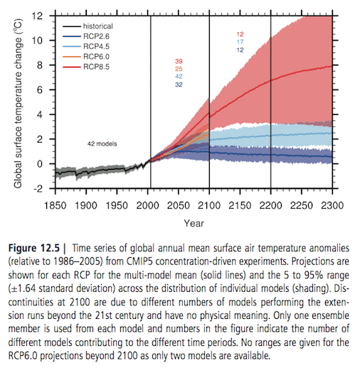
From AR5, chapter 12
Figure 1
That graph is hard to make out for 2100, here is the table of corresponding data. I highlighted RCP6.0 in 2100 – you can click to enlarge the table:
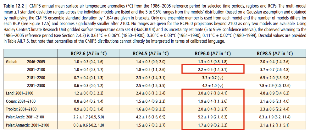
Figure 2 – Click to expand
Probabilities and Lists
The table above has a “1 std deviation” and a 5%-95% distribution. The graph (which has the same source data) has shading to indicate 5%-95% of models for each RCP scenario.
These have no relation to real probability distributions. That is, the range of 5-95% for RCP6.0 doesn’t equate to: “the probability is 90% likely that the average temperature 2080-2100 will be 1.4-3.1ºC higher than the 1986-2005 average”.
A number of climate models are used to produce simulations and the results from these “ensembles” are sometimes pressed into “probability service”. For some concept background on ensembles read Ensemble Forecasting.
Here is IPCC AR5 chapter 12:
Ensembles like CMIP5 do not represent a systematically sampled family of models but rely on self-selection by the modelling groups.
This opportunistic nature of MMEs [multi-model ensembles] has been discussed, for example, in Tebaldi and Knutti (2007) and Knutti et al. (2010a). These ensembles are therefore not designed to explore uncertainty in a coordinated manner, and the range of their results cannot be straightforwardly interpreted as an exhaustive range of plausible outcomes, even if some studies have shown how they appear to behave as well calibrated probabilistic forecasts for some large-scale quantities. Other studies have argued instead that the tail of distributions is by construction undersampled.
In general, the difficulty in producing quantitative estimates of uncertainty based on multiple model output originates in their peculiarities as a statistical sample, neither random nor systematic, with possible dependencies among the members and of spurious nature, that is, often counting among their members models with different degrees of complexities (different number of processes explicitly represented or parameterized) even within the category of general circulation models..
..In summary, there does not exist at present a single agreed on and robust formal methodology to deliver uncertainty quantification estimates of future changes in all climate variables. As a consequence, in this chapter, statements using the calibrated uncertainty language are a result of the expert judgement of the authors, combining assessed literature results with an evaluation of models demonstrated ability (or lack thereof) in simulating the relevant processes (see Chapter 9) and model consensus (or lack thereof) over future projections. In some cases when a significant relation is detected between model performance and reliability of its future projections, some models (or a particular parametric configuration) may be excluded but in general it remains an open research question to find significant connections of this kind that justify some form of weighting across the ensemble of models and produce aggregated future projections that are significantly different from straightforward one model–one vote ensemble results. Therefore, most of the analyses performed for this chapter make use of all available models in the ensembles, with equal weight given to each of them unless otherwise stated.
And from one of the papers cited in that section of chapter 12, Jackson et al 2008:
In global climate models (GCMs), unresolved physical processes are included through simplified representations referred to as parameterizations.
Parameterizations typically contain one or more adjustable phenomenological parameters. Parameter values can be estimated directly from theory or observations or by “tuning” the models by comparing model simulations to the climate record. Because of the large number of parameters in comprehensive GCMs, a thorough tuning effort that includes interactions between multiple parameters can be very computationally expensive. Models may have compensating errors, where errors in one parameterization compensate for errors in other parameterizations to produce a realistic climate simulation (Wang 2007; Golaz et al. 2007; Min et al. 2007; Murphy et al. 2007).
The risk is that, when moving to a new climate regime (e.g., increased greenhouse gases), the errors may no longer compensate. This leads to uncertainty in climate change predictions. The known range of uncertainty of many parameters allows a wide variance of the resulting simulated climate (Murphy et al. 2004; Stainforth et al. 2005; M. Collins et al. 2006). The persistent scatter in the sensitivities of models from different modeling groups, despite the effort represented by the approximately four generations of modeling improvements, suggests that uncertainty in climate prediction may depend on underconstrained details and that we should not expect convergence anytime soon.
Stainforth et al 2005 (referenced in the quote above) tried much larger ensembles of coarser resolution climate models, and was discussed in the comments of Models, On – and Off – the Catwalk – Part Four – Tuning & the Magic Behind the Scenes. Rowlands et al 2012 is similar in approach and was discussed in Natural Variability and Chaos – Five – Why Should Observations match Models?
The way I read the IPCC reports and various papers is that clearly the projections are not a probability distribution. Then the data gets inevitably gets used as a de facto probability distribution.
Conclusion
“All models are wrong but some are useful” as George Box said, actually in a quite unrelated field (i.e., not climate). But it’s a good saying.
Many people who describe themselves as “lukewarmers” believe that climate sensitivity as characterized by the IPCC is too high and the real climate has a lower sensitivity. I have no idea.
Models may be wrong, but I don’t have an alternative model to provide. And therefore, given that they represent climate better than any current alternative, their results are useful.
We can’t currently create a real probability distribution from a set of temperature prediction results (assuming a given emissions scenario).
How useful is it to know that under a scenario like RCP6.0 the average global temperature increase in 2100 has been simulated as variously 1ºC, 2ºC, 3ºC, 4ºC? (note, I haven’t checked the CMIP5 simulations to get each value). And the tropics will vary less, land more? As we dig into more details we will attempt to look at how reliable regional and seasonal temperature anomalies might be compared with the overall number. Likewise rainfall and other important climate values.
I do find it useful to keep the idea of a set of possible numbers with no probability assigned. Then at some stage we can say something like, “if this RCP scenario turns out to be correct and the global average surface temperature actually increases by 3ºC by 2100, we know the following are reasonable assumptions … but we currently can’t make any predictions about these other values..”
References
Long-term Climate Change: Projections, Commitments and Irreversibility, M Collins et al (2013) – In: Climate Change 2013: The Physical Science Basis. Contribution of Working Group I to the Fifth Assessment Report of the Intergovernmental Panel on Climate Change
Scenarios of long-term socio-economic and environmental development under climate stabilization, Keywan Riahi et al, Technological Forecasting & Social Change (2007) – free paper
Error Reduction and Convergence in Climate Prediction, Charles S Jackson et al, Journal of Climate (2008) – free paper
Notes
Note 1: As explored a little in the last article, RCP6.0 does include some changes to climate policy but it seems they are not major. I believe a very useful scenario for exploring impact assessments would be the population and development path of RCP6.0 (let’s call it RCP6.0A) without any climate policies.
For reasons of”scenario parsimony” this interesting pathway avoids attention.


It is interesting however to consider the problem from the POV of a subjective Bayesian. The RCPs are, we should note, “representative”, representative of the range of scenarios in the literature. Since each RCPs is representative of a different subsample (based on their 2100 forcings) of the scenario set assessed in AR4 it could be assumed that the relative numbers of scenarios in each subset is a reflection of expert prior information on their likelihood. On this basis RCP8.5 represented 40 scenarios; RCP6.0, 10; RCP4.5, 118; and RCP2.6, 20 (van Vuuren et al 2011). This gives at least some basis for combining the output from the 4 AR5 RCPs into a single PDF. Information on the distribution of assumptions that go into the scenarios can be added to improve the estimates e.g. the population assumption would tighten the 2100 PDF further.
This graph suggests there are a lot more scenarios around than that. Presumably most of them were post-AR4.
I think the difficulty is that scenarios are generally not created with the intention of exploring parameter space for possible outcomes. Often they’re advocating for a particular policy approach for achieving a target. I believe the reason there are a lot around the RCP4.5 area is because a lot of people are attempting to find policy pathways to produce something like RCP4.5.
SoD,
You wrote: “Models may be wrong, but I don’t have an alternative model to provide. And therefore, given that they represent climate better than any current alternative, their results are useful.”
But there is an alternative that represents climate better than the GCM’s: observation based estimates of climate sensitivity. They are done in a variety of ways, making use of differing data sets. They give fairly consistent results in the low end of the IPCC ranges: 1.0 to 1.5 K for TCR and 1.5 to 2.0 K for ECS. And they give probability distributions, unlike GCM’s.
Mike,
I didn’t comment when you wrote this comment because it’s not an area I am up to date with.
Just reading Missing iris effect as a possible cause of muted hydrological change and high climate sensitivity in models, Thorsten Mauritsen and Bjorn Stevens, Nature Goescience (2015) and they start with this:
SoD quoted a paper as saying “Equilibrium climate sensitivity to a doubling of CO2 falls between 2.0 and 4.6 K in current climate models … Inferences from the observational record, however, place climate sensitivity near the lower end of this range”.
The authors stated that incorrectly. They got the models right (although I thought it was 2.1 to 4.5 K), but the observational results are lower, mostly between 1.5 and 2.0 K. IPCC AR4 gave the range of ECS as 2.0 to 4.5 K, based on models. In AR5, the model range did not change, but IPCC expanded the range to 1.5 to 4.5 K so as to include the observations.
SOD: In the opening, you quote AR5:
“Under the assumptions of the concentration-driven RCPs, global mean surface temperatures for 2081–2100, relative to 1986–2005 will LIKELY be in the 5 to 95% range of the CMIP5 models … 2.6°C to 4.8°C (RCP8.5)”.
Here the authors are using their EXPERT JUDGMENT to describe the 90% ci for (technically “very likely”) for CMIP5 model runs as being “likely” (technically a 70% ci). What is going on here? They are guessing (probably without evidence) that the 90% ci for model output would be 2.0-5.4 °C if models did a better job of exploring parameter space. However, the high end of model output is already inconsistent with energy balance models, so it makes no sense to increase both ends of the range.
If the IPCC no longer supports 3 K is best estimate for ECS (due to the low values for ECS from energy balance models), then they shouldn’t be reporting projected warming from an ensemble of models with an average ECS of 3.3 K.
SOD writes: “Models may be wrong, but I don’t have an alternative model to provide. And therefore, given that they represent climate better than any current alternative, their results are useful.”
Part of the problem is that the IPCC practices “model democracy” – any AOGCM recommended by a member nation gets equal weight in projections of warming. If model output were weighted using a pdf from derived energy balance models, policymakers would be receiving projections that reflected all of the information we currently possess. This would be my alternative.
(One problem is that the end of this century are an intermediate regime where neither TCR nor ECS is an ideal metric. However, it should be possible to weight by TCR until CO2 accumulation slows and then gradually weight more by ECS.)
However, the high end of model output is already inconsistent with energy balance models, so it makes no sense to increase both ends of the range.
I really don’t think that’s accurate. Even Lewis and Curry 2015 showed that some reasonable baseline choices allow very high ECS (about 9.5K). Energy balance sensitivity papers have typically not addressed known biases in observations, nor known uncertainties relating to their assumption of perfect linearity between forcing and response.
I don’t see any strong case made that energy balance sensitivity tests have constrained ECS below 6C, which is already the IPCC’s very likely upper bound.
I have serious problems with having ECS much greater than TCR. That would require massive non-linearity between forcing and response. I don’t buy it. Suppose that is the case. Now consider the case where you’re in the regime of large temperature increase for small forcing. What happens if you add a new forcing? Is TCR now much higher? I don’t think so. As I said, I don’t buy it.
I have serious problems with having ECS much greater than TCR. That would require massive non-linearity between forcing and response.
I don’t think this is correct. My understanding for what sets the TCR-to-ECS ratio is really the rate at which energy is transfered from the upper ocean into the deep ocean. If this is very slow, then we will quickly warm the mixed ocean layer and atmosphere towards equilibrium, and then very slowly warm the deeper ocean until equilibrium is attained. This would mean that the ECS and TCR would be very similar, but that it would take a very long time to reach equilibrium. As the rate of energy transfer into the deep ocean increases, the TCR-to-ECS ratio would decrease – we would retain a relatively large planetary energy imbalance, and warm more slowly towards equilibrium. The TCR-to-ECS ratio would then be smaller. Given that we currently seem to be able to sustain a planetary energy imbalance of 0.5-1W/m^2 would seem to be inconsistent with a TCR-to-ECS ratio close to 1 – most estimates I’ve seen put it at around 0.7, or a bit lower.
This is discussed in Isaac Held post and also in this Hansen paper (Figure 7, in particular). I may also not have explained this all that well, so happy to be corrected/clarified if not.
DeWitt writes: “I have serious problems with having ECS much greater than TCR. That would require massive non-linearity between forcing and response.
I don’t buy it.”
ECS = F_2x*dT/(dF-dQ) (Eqn. 1)
TCR = F_2x*dT/dF) (Eqn. 2)
dQ is ocean heat uptake, dF is the change in forcing, and dT the change in temperature at some time on the path to equilibrium. F_2x is the forcing from doubled CO2. Simple algebra provides:
TCR/ECS = 1 – dQ/dF (Eqn 3)
In other works, the larger the fraction of the forcing that is going into the ocean at any time, the bigger ECS is than TCR. The massive “non-linearity” comes from simple reciprocal relationship – which is non-linear.
If you approach this from the perspective of a climate feedback parameter (L for lambda):
dW = L*dT
where dW is the change in net radiation at the TOA within a few months of fast feedbacks associated with a surface temperature change of dT. (L is less than zero by convention.) If a forcing (dF) has been applied and equilibrium warming has been reached, dW = dF. If equilibrium has NOT been reached, dW = dT – dQ. Conservation of energy means that the forcing that is not going into the ocean is going out of the TOA (with the exception of a tiny amount that is warming the atmosphere and land surface).
When dF equals F_2x, dT = TCR. If dQ = 0 and dF = dW = F_2x:
F_2x = L*ECS or L = F_2x/ECS
This provides Eqns 1 and 2. If we think more broadly, TCR can be the temperature change at the end of a doubling of CO2 that takes 7 years, 70 years, or 700 years. There is nothing special about a growth in forcing of 1% per year. Currently growth is 0.5% per year and it was 0.25% per year back in the 1960s. The slower the warming, the less deep ocean warming will lag behind the surface warming, the smaller dQ will be when forcing stops growing, and the closer “TCR” will be to ECS. Intuitively, there should be no single right answer for the difference between TCR and ECS. Equation 3 make sense mathematically and intuitively.
Frank,
The problem is that in climate models, it doesn’t work that way. If you plot temperature change vs TOA forcing, not time, you get an initial straight line, TCR. That’s fine, but later, the line almost asymptotically approaches the temperature axis. That means that a very small TOA forcing produces a very large temperature change. If heat were going into the deep ocean, the TOA forcing would not decline to a very low number. You can only get behavior like that if there is a large and increasing positive feedback at longer times. Heat going into the deep ocean doesn’t fit the bill.
See Paul_K’s article here: http://rankexploits.com/musings/2012/the-arbitrariness-of-the-ipcc-feedback-calculations/
DeWitt and ATTP: DeWitt wrote about the relationship between ECS and TCR: “The problem is that in climate models, it doesn’t work that way. If you plot temperature change vs TOA forcing, not time, you get an initial straight line, TCR.”
As best I can tell, you are not contradicting anything I wrote. You are referring to the fact that the climate feedback parameter for AOGCMs appears to change with time or Ts, a phenomena that isn’t explicitly included in my eqns: L instead of L(Ts) for example. A recent paper by Andrews (2015, J Clim) shows that global feedbacks in CMIP5 models are linear with temperature except for cloud SWR, which changes sign after about 3.5 K of warming (about 20 years) in an abrupt 4XCO2 experiment). AOGCMs differ greatly in the amount of SWR cloud feedback and its non-linearity. One model shows a change from -0.5 W/m2/K to +1.0 W/m2/K between the first 20 years of a 4X experiment and the last 130 years. See Figure 3b.
Figure 4 shows the geographic distribution feedbacks and their non-linearity.
The local climate feedback parameter increases from +1 to +5 W/m2/K in the Eastern Equatorial Pacific. However, the non-linearity of cloud SWR feedback is localized over other parts of mostly tropical oceans. The big picture is that models are projecting an accelerating runaway GHE (from +1 W/m2/K to +5 W/m2/K) mostly localized in the tropical Pacific that raises the global feedback parameter from about -2 W/m2/K today to -1 W/m2/K in the future.
Click to access jcli-d-14-00545%252E1.pdf
Looking back at my equations, if L changes with Ts, then so do BOTH ECS (= F_2x/L) and TCR (=ECS*(1-dQ/dF) change with Ts.
Anyway, a lot has been happening since Paul_K’s post at the Blackboard, Isaac Held’s early post on non-linearity, ATTP’s Hansen reference, the recognition of the discrepancy between energy balance models and AOGCMs, and some of the early explanations for the discrepancy. If he prefers, DeWitt can now say he doesn’t believe in an ACCELERATING runaway GHE in the equatorial Pacific. (:))
Frank,
The accelerating behavior is apparently based on clouds. GCM’s don’t do clouds well, to put it mildly. Of course I don’t believe in accelerating runaway greenhouse in the western Pacific. It’s a model artifact with, AFAIK, no observational evidence to support it. Needless to say, I don’t consider model behavior to be observational evidence.
DeWitt wrote: “The problem is that in climate models, it doesn’t work that way.”
I think Frank has it right. Climate models don’t work exactly like the simplified versions, but it is close enough to make the simple versions useful.
DeWitt: “If you plot temperature change vs TOA forcing, not time, you get an initial straight line, TCR. That’s fine, but later, the line almost asymptotically approaches the temperature axis.”
You are unclear here. If you are talking about what happens after a step change in forcing, then the forcing does not change with time and I don’t see how to make sense of this. It sounds like you are using “TOA forcing” to mean TOA radiative imbalance, in which case this would make sense.
DeWitt: “That means that a very small TOA forcing produces a very large temperature change. If heat were going into the deep ocean, the TOA forcing would not decline to a very low number. You can only get behavior like that if there is a large and increasing positive feedback at longer times. Heat going into the deep ocean doesn’t fit the bill.”
I don’t see how increasing positive feedback would do this either, if you mean forcing when you say forcing. But if you mean TOA radiative imbalance, then heat going into the ocean would produce exactly this behavior. Once the deep ocean is in steady state, the TOA radiative imbalance would be zero.
The Paul_K article at the blackboard appears to be very confused. In particular, he does not seem to understand that, as Frank says, “The massive “non-linearity” comes from simple reciprocal relationship – which is non-linear.”
Mike M.
Forcing is defined as the radiative imbalance at the tropopause. It isn’t a fixed quantity with time. The instantaneous forcing from a step change doesn’t change with time, but so what? It only applies at time zero. But I can call it TOA imbalance or net flux if that will make you happier.
No, it wouldn’t. You can say that again and again, but it still won’t be true. Heat going into the ocean changes the response time. It doesn’t change the sensitivity. A fixed increase in surface temperature should reduce the radiative imbalance by the same amount at any time absent a variable positive feedback. Heat going into the deep ocean doesn’t change the surface temperature very much and so doesn’t change the radiative imbalance very much.
The climate sensitivity is the change in temperature with the change in net flux. Look at Paul_K’s figure 1. Initially, a change in net flux of ~2.7 W/m² produces a surface temperature change of ~1 degree. But the TOA imbalance changes by a lot less than 1 W/m² for each of the next ~0.7 degree surface temperature changes. So the initial climate sensitivity in degrees/W/m², TCR is ~0.4. But the change in net flux to points A, B, C and D is ~0.25W/m² each, while the surface temperature changes by ~0.7 degrees for each point giving a climate sensitivity of ~3 degrees/W/m². That requires a large positive feedback in my book.
Now the slope of the straight line between the initial imbalance and zero net flux gives an ECS of ~1. But the surface temperature doesn’t follow that line, so it’s a nearly meaningless number.
DeWitt wrote: “Forcing is defined as the radiative imbalance at the tropopause. It isn’t a fixed quantity with time. The instantaneous forcing from a step change doesn’t change with time, but so what? It only applies at time zero.”
You are mistaken. It is a common mistake (you can find it at Wikipedia) that leads to a lot of confusion.
From the IPCC AR 5 glossary: “Radiative forcing is the change in the net, downward minus upward, radiative flux (expressed in W m–2) at the tropopause or top of atmosphere due to a change in an external driver of climate change, such as, for example, a change in the concentration of carbon dioxide or the output of the Sun.”
That sounds a lot like what DeWitt says, but IPCC then it goes on to add: “… radiative forcing is computed with all tropospheric properties held fixed at their unperturbed values”.
So to unpack this: A step doubling of CO2 would produce an initial imbalance of 3.7 W/m^2 at TOA. In response, surface temperature will increase and that will cause an increase in radiative emissions which, in turn, cause a reduction in the TOA imbalance. Eventually, radiative balance at TOA (i.e., equilibrium) will be restored. The temperature increase needed to restore the balance is the equilibrium climate sensitivity.
So, in the case of a step change, radiative forcing does not change with time, TOA imbalance does change with time, and the two are equal only at the time of the step change, with the limit approached from after the step change.
DeWitt wrote: “Heat going into the deep ocean doesn’t change the surface temperature very much and so doesn’t change the radiative imbalance very much.”
Energy is conserved. With the present TOA radiative imbalance, energy in exceeds energy out. That energy has to go somewhere. The only significant somewhere is the ocean. It takes five to ten years for the surface ocean temperature to change. After that, any imbalance is due to heat flux into the “deep ocean”. (Actually, mostly into the thermocline, I think; that is included in some definitions of the deep ocean and not in others.) As the ocean comes into steady state, the TOA imbalance goes to zero.
Mike M.
You still haven’t explained how energy going into the ocean, deep or otherwise, can change the ratio of ΔTs to ΔF, where F is the net flux at the TOA or tropopause.
DeWitt Payne: “You still haven’t explained how energy going into the ocean, deep or otherwise, can change the ratio of ΔTs to ΔF, where F is the net flux at the TOA or tropopause.”
I have. On any time scale of more than a few years, ΔF is equal to the net heat flux into the ocean. Thus, as the latter decreases, ΔF decreases. The ratio of ΔTs to ΔF is not, so far as I am aware, a quantity of any interest. Sounds to me like you are stuck on the mistaken idea that ΔF is the forcing.
Mike M.
It sounds like you are stuck on the idea that ΔF is meaningless. It isn’t. Again, energy going into the deeper ocean in the absence of positive feedback increases the surface temperature by only a small amount. In the absence of positive feedbacks, a one degree change in surface temperature produces a large change in ΔF. I don’t see why you can’t understand these simple ideas, but it appears pointless to waste more bandwidth.
DeWitt,
I just realized that I misunderstood something you wrote.
You wrote: “The problem is that in climate models, it doesn’t work that way. If you plot temperature change vs TOA forcing, not time, you get an initial straight line, TCR. That’s fine, but later, the line almost asymptotically approaches the temperature axis. … See Paul_K’s article here: http://rankexploits.com/musings/2012/the-arbitrariness-of-the-ipcc-feedback-calculations/“.
I translated that into something that made sense to me, but I think I now see what you meant. Here is a “Gregory plot” (scroll down to the first figure, labelled “slide 21”): https://climateaudit.org/2015/04/20/pitfalls-in-climate-sensitivity-estimation-part-3/
There is no asymptotic behavior, either in the lines or the data points. Nor should there be. It is not at all like the orange line in Paul_K’s figure 1, which he claims to be “an idealised graphic illustrating three conceptual models”. I think he just made that orange line up.
Mike M.
Perhaps he did. But then there’s also little reason to believe that the orange line in slide 21 is, in fact, the limiting behavior and that 8 degrees ΔT is the final model equilibrium temperature change. It’s an extrapolation of noisy data. If it is the limit, then TCR and ECS differ by only 20%. That’s hardly enough to worry about. For a TCR from doubling of 1.3 degrees, the ECS would be 1.6 degrees.
The scale of the y axis is odd too. I was under the impression that doubling CO2 produced a forcing of 3.7W/m². Doubling again would produce a forcing of 7.4 W/m² because the forcing is proportional to log[CO2]. But it looks like the forcing is a lot higher than that. Perhaps it was 8X CO2, not 4X. That would be 11.1W/m².
DeWitt wrote above: “Perhaps he did. But then there’s also little reason to believe that the orange line in slide 21 is, in fact, the limiting behavior and that 8 degrees ΔT is the final model equilibrium temperature change. It’s an extrapolation of noisy data. If it is the limit, then TCR and ECS differ by only 20%. That’s hardly enough to worry about. For a TCR from doubling of 1.3 degrees, the ECS would be 1.6 degrees.”
The Gregory plot of an abrupt 4X experiment doesn’t contain any information about TCR. The slope in years 1-20 is a climate feedback parameter as is the slope in years 21-150. The rate of warming can be seen in the projection of each datapoint onto the x-axis (temperature), but the data points get closer and closer together with time and multiple years are sometimes averaged. If ocean heat uptake were doubled, the rate of warming as seen by the projection of the points onto the x-axis will slow, but the slope will remain the same.
TCR/ECS = 1 – dQ/dF.
Are you willing to broaden your concept of TCR to experiments where warming from a forcing increasing at something different from 1% per year. If so, you could apply this formula at any time point in an abrupt 4X experiment. The transient warming at any time along the path to equilibrium depends on what fraction of the forcing is being taken up by the ocean (rather than leaving the planet as radiative cooling through the TOA.
Sorry I missed these replies until now.
Paulski0 wrote: “Even Lewis and Curry 2015 showed that some reasonable baseline choices allow very high ECS (about 9.5K).”
This is incorrect. Lewis and Curry (2014) reports an ECS of 1.64 K with a 95% ci of 1.05-4.05 K using the IPCC’s values for warming and forcing from a base period of 1859-1882 to a final period of 1995-2011. Using a base period of 1930-1950 and the same final period, the best estimate for ECS is similar (1.72 K) but the 95% ci is wider (0.90-9.45K). The hypothesis that ECS could be substantial greater than 4 K and as high as 9.5 K is inconsistent with the data from the longer period and therefore wrong.
In conventional science, a theory can be consistent with a dozen experiments – but if it is inconsistent with one other experiment, the theory has been invalidated (as long as the experiment is believed to be correct). Lewis and Curry believe the analysis of the longer period is right and therefore nothing in their paper supports an ECS of 9.5 K. The highest value in their abstract is 4.05 K.
In the introduction, they discuss earlier work where older values about forcing, warming and ocean heat uptake produced higher values for ECS. Those input values are now considered to be obsolete by the IPCC – especially the lower limit for negative forcing from aerosols – so these older experiments don’t invalidate Lewis and Curry.
Using narrow limits for aerosol forcing published by B. Stevens, Lewis has calculated and a much narrower and lower 95% ci for ECS (1.05-2.2 K). Since Stevens’ value for aerosol forcing isn’t accepted as superior to earlier values (say by the IPCC), the hypothesis that ECS is between 2.5 and 4 K isn’t inconsistent with experiment right now.
I have read this Blog avidly for many years, this new series really is excellent.
Looking forward to the next instalment.
Thanks for an encyclopaedic website/blog, I am a new reader and grateful for the content. Regarding storage of the 90%+ of GW heat in the oceans and that heat’s contribution to global circulation patterns and currents, I wonder whether there is sufficient data available regarding undersea volcanic activity including degassing and whether this aspect is getting sufficient consideration in the calculations of ocean warming because it seems to me that it could be very significant in the whole scheme of things.
Mike,
Heat transfer from the Earth’s core is not evenly distributed. But over large areas, it averages out to a small number, a few tenths of a watt per square meter. Pretty much the same goes for volcanic CO2. It’s a small fraction of current human emissions. Over time spans of hundreds of thousands of years or longer, the geologic carbon cycle, weathering of silicate rocks to form carbonates, subduction of carbonates and conversion of carbonates back to silicates with evolution of CO2, dominates. Look at the PETM, for example.
https://en.wikipedia.org/wiki/Paleocene%E2%80%93Eocene_Thermal_Maximum
DeWitt: Doesn’t analysis of magma and volcanic rock tell us how much energy is being released by radioactive decay per unit volume inside the Earth? If so, assuming a steady state, we know the rate at which heat is escaping from inside the Earth. This doesn’t mean that we can’t be living in a geological era when that steady state has been disturbed.
See: https://en.wikipedia.org/wiki/Earth%27s_internal_heat_budget
47TW from the core compared to 173,000TW from insolation.
DeWItt and Mike: Starting fresh, DeWitt wrote:
“The accelerating behavior is apparently based on clouds. GCM’s don’t do clouds well, to put it mildly. Of course I don’t believe in accelerating runaway greenhouse in the western Pacific. It’s a model artifact with, AFAIK, no observational evidence to support it. Needless to say, I don’t consider model behavior to be observational evidence.”
It’s too bad the Blackboard isn’t keeping up; your reply seems obsolete. Can we discuss this from the perspective of the climate feedback parameter (which is sometimes called lambda (L) and other times alpha)? Imagine a chaotic and persistent change in upwelling of cold deep water and downwelling of warm surface water caused GMST to warm 1 K – without any change in radiative forcing.
dW = L*dT
This will cause a change in the amount thermal radiation emitted to space (Planck feedback) and it will be modified by the other fast feedbacks. The sum of all these feedbacks is the climate feedback parameter (L, with a negative value representing an increase in LWR emitted to space and SWR reflected to space). L is a fundamental property of our planet that is independent of any forcing.
Now let’s imagine warming caused by a change in forcing, dF (either gradual or abrupt) and the temperature change (dT) associated with it. If equilibrium has been restored by a temperature change, then dW + dF = 0. To calculate ECS (K/doubling), divide F_2x (W/m2/doubling) by L (W/m2/K). If L is -1 W/m2/K, ECS is 3.7 K (high climate sensitivity). If L is -2 W/m2/K, climate sensitivity is 1.85 K, roughly that exhibited by energy balance models. If L is -3 or less W/m2/K, ECS is less than 1.2 K and there is no amplification from feedbacks. And, if L is zero or greater, a runaway greenhouse effect exists.
Using climate models, we can cause a temperature change in the absence of forcing. (This is one way of determining the no-feedbacks climate sensitivity.) When models were constrained to follow the rise in SST from 1979 to 2011 without any change in forcing (roughly the period studied by Otto (2013) with EBM’s), the increase in net flux across the TOA (2.3 W/m2/K) was consistent with the low climate sensitivity reported by Otto.
In other words, the atmospheric modules of AOGCMs – with their poor clouds, lack of a hot-spot in the upper tropical troposphere, and many other flaws – agree with EBMs about the current climate feedback parameter.
http://onlinelibrary.wiley.com/doi/10.1002/2016GL068406/abstract;jsessionid=83CDBC898B6180BBBDE40019743759C6.f02t02
Andrews (2016), recommended by Nic Lewis: “We investigate the climate feedback parameter α (W m−2 K−1) during the historical period (since 1871) in experiments using the HadGEM2 and HadCM3 atmosphere general circulation models (AGCMs) with constant preindustrial atmospheric composition and time-dependent observational sea surface temperature (SST) and sea ice boundary conditions. In both AGCMs, for the historical period as a whole, the effective climate sensitivity is ∼2 K (α≃1.7 W m−2 K−1), and α shows substantial decadal variation caused by the patterns of SST change. Both models agree with the AGCMs of the latest Coupled Model Intercomparison Project in showing a considerably smaller effective climate sensitivity of ∼1.5 K (α = 2.3 ± 0.7 W m−2 K−1), given the time-dependent changes in sea surface conditions observed during 1979–2008, than the corresponding coupled atmosphere-ocean general circulation models (AOGCMs) give under constant quadrupled CO2 concentration. These findings help to relieve the apparent contradiction between the larger values of effective climate sensitivity diagnosed from AOGCMs and the smaller values inferred from historical climate change.”
DeWitt and Mike: So why does the IPCC report much higher values for ECS from AOGCMs than from EBMs?
Answer: The climate feedback parameter changes with temperature. In the abrupt 4XCO2 experiments used to calculate ECS, many models show a change in the slope (L, W/m2/K) of the Gregory plot (radiative imbalance vs temperature) after about 20 years, when the planet has warmed by about 3.5 K. L before this change is consistent with low climate sensitivity and L after this change is consistent with high climate sensitivity. The factor that changes the most globally is SWR feedback from cloudy skies. Through the first few degrees of warming, SWR cloud feedback is negative, then it turns positive.
Using models you can also look at local feedback. How do TOA OLR and reflected SWR change over a particular location as surface temperature changes? Are these changes in LWR or SWR and do they come from clear or cloudy skies. In the first 20 years of an abrupt 4X experiment, the local climate feedback parameter is negative in most places, around zero in the tropical Pacific and averages about 2 W/m2/K globally (low climate sensitivity). After 20 years, the local climate feedback parameter in the tropics has risen to +5 W/m2/K and globally it rises to around 1 W/m2/K (high climate sensitivity). If that happened globally, there would be a runaway GHE. This presumably lead to dramatically more heat transport out of the tropics. (It isn’t escaping to space.)
All of the stuff about the climate feedback parameter is irrelevant to TCR and ocean heat uptake. If more heat goes into the ocean, warming is slow. That means the annual data points on the Gregory plot are closer together, but the heat flux into the deep ocean doesn’t change the relationship dW = k*dT. Ocean heat uptake is only important when you want to calculate ECS from transient warming.
Andrews (2015), also recommended by Nic. http://centaur.reading.ac.uk/38318/8/jcli-d-14-00545%252E1.pdf
“Experiments with CO2 instantaneously quadrupled and then held constant are used to show that the relationship between the global-mean net heat input to the climate system and the global-mean surface air temperature change is nonlinear in phase 5 of the Coupled Model Intercomparison Project (CMIP5) atmosphere–ocean general circulation models (AOGCMs). The nonlinearity is shown to arise from a change in strength of climate feedbacks driven by an evolving pattern of surface warming. In 23 out of the 27 AOGCMs examined, the climate feedback parameter becomes significantly (95% confidence) less negative (i.e., the effective climate sensitivity increases) as time passes. Cloud feedback parameters show the largest changes. In the AOGCM mean, approximately 60% of the change in feedback parameter comes from the tropics (30N–30S). An important region involved is the tropical Pacific, where the surface warming intensifies in the east after a few decades. The dependence of climate feedbacks on an evolving pattern of surface warming is confirmed using the HadGEM2 and HadCM3 atmosphere GCMs (AGCMs). With monthly evolving sea surface temperatures and sea ice prescribed from its AOGCM counterpart, each AGCM reproduces the time-varying feedbacks, but when a fixed pattern of warming is prescribed the radiative response is linear with global temperature change or nearly so. It is also demonstrated that the regression and fixed-SST methods for evaluating effective radiative forcing are in principle different, because rapid SST adjustment when CO2 is changed can produce a pattern of surface temperature change with zero global mean but nonzero change in net radiation at the top of the atmosphere (-0.5 W/m2 in HadCM3).”
The global climate feedback parameter is a composite of a regional climate feedback parameters. Since different locations warm at different rates due to differences in ocean heat uptake, a non-linear Gregory plot doesn’t mean local climate feedback parameters must be non-linear. A non-linear Gregory plot could be caused by more rapid ocean heat uptake delaying warming in regions with a low climate feedback parameter. At his blog, Held suggested that this could happen at high latitudes. Unfortunately, the big changes are in the tropics, where heat uptake into the deep ocean is slowest.
Frank,
Just because models may give the same behavior as EBM’s in the short term does not mean that long term model behavior has anything to do with reality, especially when clouds are involved.
Frank,
To put it another way: Even though what’s happening in the real world isn’t an instantaneous 2X or 4X CO2 change, CO2 has been changing long enough that the non-linearity should be showing up. That’s probably why the models are running so hot compared to the real world.
Franks,
Thanks for the references. They look interesting.
In particular, Gregory and Andrews (2016) looks like the sort of diagnostic test that modellers ought to be doing. Note that in the abstract you cite they say “”In both AGCMs, for the historical period as a whole, the effective climate sensitivity is ∼2 K (α≃1.7 W m−2 K−1), and α shows substantial decadal variation caused by the patterns of SST change.”
That is less than the normal model sensitivity, so it sounds like they tuned the model to get the correct forcing. I will have to dig into the details.
You wrote: “The climate feedback parameter changes with temperature.”
But almost all the models in AR5 show that 4xCO2 gives very nearly twice the warming of 2xCO2; that indicates little non-linearity up to 4xCO2.
You wrote: “In the abrupt 4XCO2 experiments used to calculate ECS, many models show a change in the slope (L, W/m2/K) of the Gregory plot (radiative imbalance vs temperature) after about 20 years, … The factor that changes the most globally is SWR feedback from cloudy skies.”
I am not sure what that means, since the slope has to change as the new equilibrium is approached. Any direct effect of clouds occurs in weeks or months, rather than decades. And the time scale suggests that the ocean is involved. So it sounds like changes in sea surface T cause changes in clouds resulting in a delayed feedback. Interesting, and makes sense; I will have to dig into the paper. But the models suck at clouds, so maybe it is correct or maybe not.
Note that direct flows of heat in/out of the deep ocean are too small for variations in those flows to cause a direct climate effect. Phenomena like El Nino likely cause warming by changing cloud patterns
Mike & DeWItt: Is this the AR5 reference for 2X and 4X experiments? If so, these are EMIC’s (intermediate complexity) not AOGCMs.
https://www.ipcc.ch/pdf/assessmentreport/ar5/wg1/WG1AR5_Chapter09_FINAL.pdf Table 9.6, p 821.
I don’t know if the non-linearity develops with time or with temperature, but the latter made more sense to me before you pointed out these results from EMICs. Nic Lewis commented on some of these paper at Judy’s recently. They seem to rule out some of the proposed reasons why EBM’s might be wrong: 1) The cooling effects of aerosols are delayed because they mostly cool regions dominated by downward ocean heat uptake rather than upward convection. 2) The effective radiative forcing we have experienced is smaller than used by Otto (2013) and by L&C (2104).
ttps://judithcurry.com/2017/04/18/how-inconstant-are-climate-feedbacks-and-does-it-matter/
I’ve tried convincing Nic that abrupt 4X experiments aren’t reliable because the abrupt warming produces an stably stratified ocean that won’t occur in the real world. He has insisted (correctly) that ocean heat uptake only effects TCR and that the low climate feedback parameter in the early years of abrupt 4X experiments and in 1% pa runs (TCR) supports the results from EBM’s. Now belief in high ECS may require accepting a radical shift that most models experience to varying extents in the distant future. Today, both EBMs and models say climate sensitivity is low NOW. What evidence can possibly validate a change in the future?
Others, of course, may not see it this way. Certainly, characterizing this as an accelerating runaway GHE in the equatorial Pacific is somewhat of an exaggeration. Less heat is escaping to space as SSTs warm, but that presumably means that poleward transport increases.
DeWItt: All models are wrong. However, they may be useful in characterizing a high climate feedback parameter today, even if they may be increasingly wrong in the 22nd century.
Frank,
Yes, I was referring to Table 9.6 in AR5. I had forgotten that those are for EMIC’s.
You wrote: “I don’t know if the non-linearity develops with time or with temperature, but the latter made more sense to me before you pointed out these results from EMICs.”
I think there are two questions here. One is whether the equilibrium temperature change is linear in forcing. I think that is generally accepted as very likely, at least for modest forcing, and that is what is shown by the EMIC’s. If that is so then there is the question of whether the non-linear time evolution is due to time or temperature. If the former, then it would not seem to be an issue other than in step change models; if the latter, then the models would imply that a nasty surprise may be waiting. In that case, I am sure that those who want to discredit the observational ECS results would be shouting it from the rooftops. The way to tell would be to compare the time evolution after a 2xCO2 step change to a 4xCO2 change. That has certainly been done.
Nic Lewis commented on some of these paper at Judy’s recently. They seem to rule out some of the proposed reasons why EBM’s might be wrong: 1) The cooling effects of aerosols are delayed because they mostly cool regions dominated by downward ocean heat uptake rather than upward convection. 2) The effective radiative forcing we have experienced is smaller than used by Otto (2013) and by L&C (2104).
ttps://judithcurry.com/2017/04/18/how-inconstant-are-climate-feedbacks-and-does-it-matter/
You wrote: “I’ve tried convincing Nic that abrupt 4X experiments aren’t reliable because the abrupt warming produces an stably stratified ocean that won’t occur in the real world.”
But the ocean is mostly stably stratified. The basic circulation should not change at long as there are sufficiently cold areas at the surface to produce cold deep water. But an abrupt change will surely produce all sorts of unrealistic transients, so I would think that such models would be only useful for the asymptotic result.
You wrote: “He has insisted (correctly) that ocean heat uptake only effects TCR ”
That seems to be the usual belief among modellers, but I am skeptical. The oceans are more than just a big heat sink. They play a significant role in transporting heat. I would think that ocean currents are an important factor in patterns of cloudiness. Since clouds have such large radiative effects, internal ocean dynamics could cause changes in radiative forcing and, therefore, climate change. Climate variability shows red noise behavior on time scales longer than roughly 10^2 years. What causes that? Whatever it is,It is not in the models. My guess is chaotic dynamics in the ocean.
You wrote: “both EBMs and models say climate sensitivity is low NOW. What evidence can possibly validate a change in the future?”
A good question. I don’t think it can be answered without first establishing a good understanding of climate change in the past.
Mike M: Next time he posts somewhere, I’ll try to remember to ask Nic about differences between 2X and 4X runs, both abrupt and gradual. It suddenly occurs to me that time could be an important variable if acceleration of an ocean current is what leads to a change in the climate feedback parameter. It is possible both an abrupt 2X and 4X experiment could bend after about the same number of years, because that is how long if takes to change the velocity of a large mass of water.
Oceans are more than just a big heat sink. Every column of grid cells has its own local climate feedback parameter – modified by heat transport into and out of the column at different levels. The global climate feedback parameters is the sum of all of these local processes and if the local temperature change isn’t correct, then the feedback will also be incorrect.
I’m somewhat confused about ocean heat uptake because it seems to involve at least two phenomena: deep water formation (which may resemble a conveyor belt, not diffusion) and eddy diffusion. As the planet warms, is deepwater being formed from surface water that is warmer than it formerly was? Or does the temperature of surface water need to be just as cold as it used to be in order to be dense enough to sink? Elsewhere, ocean heat uptake is supposed to follow isopycnals, and these will have less slope when the ocean is more stably stratified. I need to find some good references about this subject.
Frank,
It seems hard to find anything thorough on ocean heat uptake. I’ve only found pieces and have had to fill in some gaps myself, so I may be mistaken in some of my conclusions. One thing that is confusing is the terminology. In some contexts, “deep ocean” is everything below the mixed layer and in others it is below the thermocline.
Diffusion of heat across the thermocline clearly transfers heat downward. So I think that the overturning circulation transfers heat out of the deep ocean and keeps it cold. I have read that the temperature of the deep ocean is determined largely by the coldest parts of the surface ocean; that makes physical sense. So an increase in average temperature at the surface should not directly affect the temperature of the deep ocean, as long as there are places and times where sea ice can form.
An increase in surface temperature would increase the gradient across the thermocline, so that might increase heat transfer into the deep ocean and cause a bit more warming of water as it travels from areas of deep water formation to areas of upwelling. But a larger T gradient would increase stability and reduce eddy diffusion. So that would reduce heat transfer into the deep ocean. My guess is that the net effect would be small. I suspect that the main warming would be within the thermocline, rather than the deep water. I think that is consistent with the time scale for reaching steady state, which seems to be a few centuries rather than millennia.
Mike M.
My understanding is that if the surface warms, the thermocline moves down. The depth of the thermocline is determined by the balance between heat carried downward by eddy diffusion and cold water upwelling. That’s off the top of my head, so I could be mistaken about the details.
That leads me to believe that there isn’t a mechanism to transfer excess solar energy below the thermocline. So the people who claim that the ‘missing’ heat is going into the ocean below 2000m are probably wrong. Again, that’s my opinion and I’m open to being proved wrong.