The subject of EMICs – Earth Models of Intermediate Complexity – came up in recent comments on Ghosts of Climates Past – Eleven – End of the Last Ice age. I promised to write something about EMICs, in part because of my memory of a more recent paper on EMICs. This article will just be short as I found that I have already covered some of the EMIC ground.
In the previous 19 articles of this series we’ve seen a concise summary (just kidding) of the problems of modeling ice ages. That is, it is hard to model ice ages for at least three reasons:
- knowledge of the past is hard to come by, relying on proxies which have dating uncertainties and multiple variables being expressed in one proxy (so are we measuring temperature, or a combination of temperature and other variables?)
- computing resources make it impossible to run a GCM at current high resolution for the 100,000 years necessary, let alone to run ensembles with varying external forcings and varying parameters (internal physics)
- lack of knowledge of key physics, specifically: ice sheet dynamics with very non-linear behavior; and the relationship between CO2, methane and the ice age cycles
The usual approach using GCMs is to have some combination of lower resolution grids, “faster” time and prescribed ice sheets and greenhouse gases.
These articles cover the subject:
Part Seven – GCM I – early work with climate models to try and get “perennial snow cover” at high latitudes to start an ice age around 116,000 years ago
Part Eight – GCM II – more recent work from the “noughties” – GCM results plus EMIC (earth models of intermediate complexity) again trying to produce perennial snow cover
Part Nine – GCM III – very recent work from 2012, a full GCM, with reduced spatial resolution and speeding up external forcings by a factors of 10, modeling the last 120 kyrs
Part Ten – GCM IV – very recent work from 2012, a high resolution GCM called CCSM4, producing glacial inception at 115 kyrs
One of the the papers I thought about covering in this article (Calov et al 2005) is already briefly covered in Part Eight. I would like to highlight one comment I made in the conclusion of Part Ten:
What the paper [Jochum et al, 2012] also reveals – in conjunction with what we have seen from earlier articles – is that as we move through generations and complexities of models we can get success, then a better model produces failure, then a better model again produces success. Also we noted that whereas the 2003 model (also cold-biased) of Vettoretti & Peltier found perennial snow cover through increased moisture transport into the critical region (which they describe as an “atmospheric–cryospheric feedback mechanism”), this more recent study with a better model found no increase in moisture transport.
So, onto a little more about EMICs.
There are two papers from 2000/2001 describing the CLIMBER-2 model and the results from sensitivity experiments. These are by the same set of authors – Petoukhov et al 2000 & Ganopolski et al 2001 (see references).
Here is the grid:
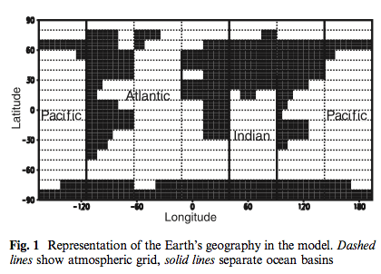
From Petoukhov et al (2000)
The CLIMBER-2 model has a low spatial resolution which only resolves individual continents (subcontinents) and ocean basins (fig 1). Latitudinal resolutions is the same for all modules (10º). In the longitudinal direction the Earth is represented by seven equal sectors (roughly 51º longitude) in the atmosphere and land modules.
The ocean model is a zonally averaged multibasin model, which in longitudinal direction resolves only three ocean basins Atlantic, Indian, Pacific). Each ocean grid cell communicates with either one, two or three atmosphere grid cells, depending on the width of the ocean basin. Very schematic orography and bathymetry are prescribed in the model, to represent the Tibetan plateau, the high Antarctic elevation and the presence of the Greenland-Scotland sill in the Atlantic ocean.
The atmospheric model has a simplified approach, leading to the description 2.5D model. The time step can be relaxed to about 1 day per step. The ocean grid is a little finer in latitude.
On selecting parameters and model “tuning”:
Careful tuning is essential for a new model, as some parameter values are not known a priori and incorrect choices of parameter values compromise the quality and reliability of simulations. At the same time tuning can be abused (getting the right results for the wrong reasons) if there are too many free parameters. To avoid this we adhered to a set of common-sense rules for good tuning practice:
1. Parameters which are known empirically or from theory must not be used for tuning.
2. Where ever possible parametrizations should be tuned separately against observed data, not in the context of the whole model. (Most of the parameters values in Table 1 were obtained in this way and only few of them were determined by tuning the model to the observed climate).
3. Parameters must relate to physical processes, not to specific geographic regions (hidden flux adjustments).
4. The number of tuning parameters must be much smaller than the degrees of freedom predicted by the model. (In our case the predicted degrees of freedom exceed the number of tuning parameters by several orders of magnitude).
To apply the coupled climate model for simulations of climates substantially different from the present, it is crucial to avoid any type of ̄flux adjustment. One of the reasons for the need of ̄flux adjustments in many general circulation models is their high computational cost, which makes optimal tuning difficult. The high speed of CLIMBER-2 allows us to perform many sensitivity experiments required to identify the physical reasons for model problems and the best parameter choices. A physically correct choice of model parameters is fundamentally different from a flux adjustment; only in the former case the surface fluxes are part of the proper feedbacks when the climate changes.
Note that many GCMs back in 2000 did need to use flux adjustment (in Natural Variability and Chaos – Three – Attribution & Fingerprints I commented “..The climate models “drifted”, unless, in deity-like form, you topped up (or took out) heat and momentum from various grid boxes..)
So this all sounds reasonable. Obviously it is a model with less resolution than a GCM, and even the high resolution (by current standards) GCMs need some kind of approach to parameter selection (see Models, On – and Off – the Catwalk – Part Four – Tuning & the Magic Behind the Scenes).
What I remembered about EMICs and suggested in my comment was based on this 2010 paper by Ganopolski, Calov & Claussen:
We will start the discussion of modelling results with a so-called Baseline Experiment (BE). This experiment represents a “suboptimal” subjective tuning of the model parameters to achieve the best agreement between modelling results and palaeoclimate data. Obviously, even with a model of intermediate complexity it is not possible to test all possible combinations of important model parameters which can be considered as free (tunable) parameters.
In fact, the BE was selected from hundred model simulations of the last glacial cycle with different combinations of key model parameters.
Note, that we consider “tunable” parameters only for the ice-sheet model and the SEMI interface, while the utilized climate component of CLIMBER-2 is the same in previous studies, such as those used by C05 [this is Calov et al. (2005)]. In the next section, we will discuss the results of a set of sensitivity experiments, which show that our modelling results are rather sensitive to the choice of the model parameters..
..The ice sheet model and the ice sheet-climate interface contain a number of parameters which are not derived from first principles. They can be considered as “tunable” parameters. As stated above, the BE was subjectively selected from a large suite of experiments as the best fit to empirical data. Below we will discuss results of a number of additional experiments illustrating the sensitivity of simulated glacial cycle to several model parameters. These results show that the model is rather sensitive to a number of poorly constrained parameters and parameterisations, demonstrating the challenges to realistic simulations of glacial cycles with a comprehensive Earth system model.
And in their conclusion:
Our experiments demonstrate that the CLIMBER-2 model with an appropriate choice of model parameters simulates the major aspects of the last glacial cycle under orbital and greenhouse gases forcing rather realistically. In the simulations, the glacial cycle begins with a relatively abrupt lateral expansion of the North American ice sheets and parallel growth of the smaller northern European ice sheets. During the initial phase of the glacial cycle (MIS 5), the ice sheets experience large variations on precessional time scales. Later on, due to a decrease in the magnitude of the precessional cycle and a stabilising effect of low CO2 concentration, the ice sheets remain large and grow consistently before reaching their maximum at around 20 kyr BP..
..From about 19 kyr BP, the ice sheets start to retreat with a maximum rate of sea level rise reaching some 15 m per 1000 years around 15kyrBP. The northern European ice sheets disappeared first, and the North American ice sheets completely disappeared at around 7 kyr BP. Fast sliding processes and the reduction of surface albedo due to deposition of dust play an important role in rapid deglaciation of the NH. Thus our results strongly support the idea about important role of aeolian dust in the termination of glacial cycles proposed earlier by Peltier and Marshall (1995)..
..Results from a set of sensitivity experiments demonstrate high sensitivity of simulated glacial cycle to the choice of some modelling parameters, and thus indicate the challenge to perform realistic simulations of glacial cycles with the computationally expensive models.
My summary – the simplifications of the EMIC combined with the “trying lots of parameters” approach means I have trouble putting much significance on the results.
While the basic setup, as described in the 2000 & 2001 papers seems reasonable, EMICs miss a lot of physics. This is important with something like starting and ending an ice age, where the feedbacks in higher resolution models can significantly reduce the effect seen by lower resolution models. When we run 100’s of simulations with different parameters (relating to the ice sheet) and find the best result I wonder what we’ve actually found.
That doesn’t mean they are of no value. Models help us to understand how the physics of climate actually works, because we can’t do these calculations in our heads. GCMs require too much computing resources to properly study ice ages.
So I look at EMICs as giving some useful insights that need to be validated with more complex models. Or with further study against other observations (what predictions do these parameter selections give us that can be verified?)
I don’t see them as demonstrating that the results “show” we’ve now modeled ice ages. The exact same comment also goes for another 2007 paper which used a GCM coupled to an ice sheet model that we covered in Part Nineteen – Ice Sheet Models I. An update of that paper in 2013 came with a excited Nature press release but to me simply demonstrates that with a few unknown parameters you can get a good result with some specific values of those parameters. This is not at all surprising. Let’s call it a good start.
Perhaps Abe Ouchi et al 2013 was the paper that will be verified as the answer to the question of ice age terminations – the delayed isostatic rebound.
Perhaps Ganopolski, Calov & Claussen 2010 with the interaction of dust on ice sheets will be verified as the answer to that question.
Perhaps neither will be.
Articles in this Series
Part One – An introduction
Part Two – Lorenz – one point of view from the exceptional E.N. Lorenz
Part Three – Hays, Imbrie & Shackleton – how everyone got onto the Milankovitch theory
Part Four – Understanding Orbits, Seasons and Stuff – how the wobbles and movements of the earth’s orbit affect incoming solar radiation
Part Five – Obliquity & Precession Changes – and in a bit more detail
Part Six – “Hypotheses Abound” – lots of different theories that confusingly go by the same name
Part Seven – GCM I – early work with climate models to try and get “perennial snow cover” at high latitudes to start an ice age around 116,000 years ago
Part Seven and a Half – Mindmap – my mind map at that time, with many of the papers I have been reviewing and categorizing plus key extracts from those papers
Part Eight – GCM II – more recent work from the “noughties” – GCM results plus EMIC (earth models of intermediate complexity) again trying to produce perennial snow cover
Part Nine – GCM III – very recent work from 2012, a full GCM, with reduced spatial resolution and speeding up external forcings by a factors of 10, modeling the last 120 kyrs
Part Ten – GCM IV – very recent work from 2012, a high resolution GCM called CCSM4, producing glacial inception at 115 kyrs
Pop Quiz: End of An Ice Age – a chance for people to test their ideas about whether solar insolation is the factor that ended the last ice age
Eleven – End of the Last Ice age – latest data showing relationship between Southern Hemisphere temperatures, global temperatures and CO2
Twelve – GCM V – Ice Age Termination – very recent work from He et al 2013, using a high resolution GCM (CCSM3) to analyze the end of the last ice age and the complex link between Antarctic and Greenland
Thirteen – Terminator II – looking at the date of Termination II, the end of the penultimate ice age – and implications for the cause of Termination II
Fourteen – Concepts & HD Data – getting a conceptual feel for the impacts of obliquity and precession, and some ice age datasets in high resolution
Fifteen – Roe vs Huybers – reviewing In Defence of Milankovitch, by Gerard Roe
Sixteen – Roe vs Huybers II – remapping a deep ocean core dataset and updating the previous article
Seventeen – Proxies under Water I – explaining the isotopic proxies and what they actually measure
Eighteen – “Probably Nonlinearity” of Unknown Origin – what is believed and what is put forward as evidence for the theory that ice age terminations were caused by orbital changes
Nineteen – Ice Sheet Models I – looking at the state of ice sheet models
References
CLIMBER-2: a climate system model of intermediate complexity. Part I: model description and performance for present climate, V Petoukhov, A Ganopolski, V Brovkin, M Claussen, A Eliseev, C Kubatzki & S Rahmstorf, Climate Dynamics (2000)
CLIMBER-2: a climate system model of intermediate complexity. Part II: model sensitivity, A Ganopolski, V Petoukhov, S Rahmstorf, V Brovkin, M Claussen, A Eliseev & C Kubatzki, Climate Dynamics (2001)
Transient simulation of the last glacial inception. Part I: glacial inception as a bifurcation in the climate system, Reinhard Calov, Andrey Ganopolski, Martin Claussen, Vladimir Petoukhov & Ralf Greve, Climate Dynamics (2005)
Simulation of the last glacial cycle with a coupled climate ice-sheet model of intermediate complexity, A. Ganopolski, R. Calov, and M. Claussen, Climate of the Past (2010)


