A few people have asked about the fascinating 2006 paper by Gerard Roe, In defense of Milankovitch.
Roe’s paper appears to show an excellent match between the rate of change of ice volume and insolation at 65°N in June. I’ve been puzzled by the paper for a while, because if this value of insolation does successfully predict changes in ice volume then case closed. Except we struggle to match glacial terminations with insolation (see earlier posts like Part Thirteen, Twelve, Eleven – End of the Last Ice age).
And we should also expect to find a 100 kyr period in the 65°N insolation spectrum. But we don’t.
To be fair to Roe, he does state:
The Milankovitch hypothesis as formulated here does not explain the large rapid deglaciations that occurred at the end of some of the ice age cycles
[Emphasis added].
To be critical, it doesn’t seem like anyone is disputing that ice sheets wax and wane with at least some attachment to 40k (obliquity) and 20k (precession) cycles so what exactly does the paper demonstrate that is new? The missing bit of the puzzle is why ice ages start and end.
On the plus side, Roe points out:
Surprisingly, the [Milankovitch] hypothesis remains not clearly defined..
Which is the same point I made in Ghosts of Climates Past – Part Six – “Hypotheses Abound”.
One of the reasons I’ve spent quite a bit of time collecting and understanding datasets – see Part Fourteen – Concepts & HD Data – was for this kind of problem. Roe’s figure 2 spans half a page but covers 800,000 years. With the thick lines used I can’t actually tell if there is a match, and being poor at real statistics I want to see the data rather than just accept a correlation.
There’s not much point comparing SPECMAP (or LR04) with insolation because both of these datasets are “tuned” to summer 65°N insolation. If we find success then we accept that the producers of the dataset were competent in their objective. If we find lack of success we have to write to them with bad news. No one wants to do that.
Fortunately we have an interesting dataset from Peter Huybers (2007). This is an update of HW04 (Huybers & Wunsch 2004) which created a proxy for global ice volume from deep ocean cores without “orbital tuning”. It’s based on an autocorrelated sedimentation model, requiring that key turning points from many different cores all occur at the same time, and a key dateable event at around 800,000 years ago that shows up in most cores.
Some readers are wondering:
Why not use the ice cores you have been writing about?
Good question. The oxygen isotope (δ18O), or deuterium isotope (δD), in the ice is more a measure of local temperature than anything else (and it’s complicated). So Greenland and Antarctic ice cores provide lots of useful data, but not global ice volume. For that, we need to capture the δ18O stored in deep ocean sediments. The δ18O in deep ocean cores, to a first order, appears to be a measure of the amount of water locked up in global ice sheets. However, we have no easy way to objectively date the ocean cores, so some assumptions are needed.
Fortunately, Roe compared his theory with two datasets, the famous SPECMAP (warning, orbital tuning was used in the creation of this dataset) and HW04:
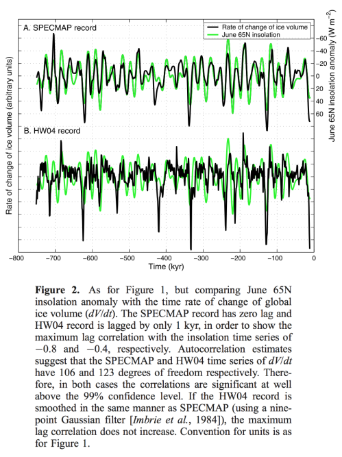
Figure 1
I downloaded the updated Huybers 2007 dataset. It is in 1 kyr intervals. I have calculated the insolation at all latitudes and all days for the last 500 kyrs using Jonathan Levine’s MATLAB program. This is also in 1 kyrs intervals. I used the values at 65N and June 21st (day 172 – thanks Climateer, for helping me with the basics of calendar days!).
I calculated change in ice volume in a very simple way – (value at time t+1 – value at time t) divided by time change. I scaled the resulting dataset to the same range as the insolation anomalies – so that they plot nicely. And I plotted insolation anomaly = mean(insolation) – insolation:
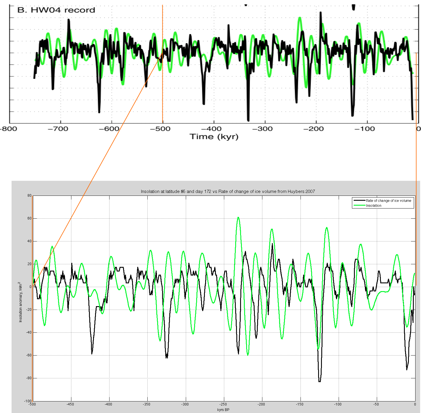
Figure 2 – Click to Expand
The two sets of data look very similar over the last 500 kyrs. I assume that some minor changes, e.g., at about 370 kyrs, are due to dataset updates. Note that insolation anomaly is effectively inverted to help match trends by eye – high insolation should lead to negative change in ice volume and vice-versa.
For reference, here is my calculation on its own (click to get the large version):
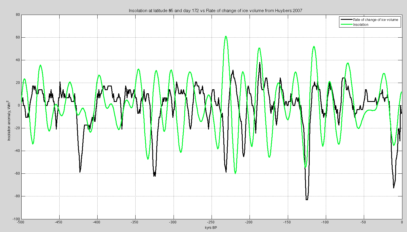
Figure 3 – Click to Expand
I did a Pearson correlation between the two datasets and obtained 0.08. That is, very little correlation. This just tells us what we can see from looking at the graph – the two key values are in phase to begin with then move out of phase and back into phase by the end.
Correlation between 0-100 kyrs: 0.66 (great)
Correlation between 101-200 kyrs: 0.51 (great)
Correlation between 201-300 kyrs: -0.72 (wrong direction)
Correlation between 301-400 kyrs -0.27 (wrong direction)
Correlation between 401-500 kyrs: 0.18 (wavering)
I also did a Spearman rank correlation (correlates the rank of the two datasets to make it resistance to outliers) = 0.09, and just because I could, a Kendall correlation as well = 0.07.
I’m a bit of a statistics amateur so comparing datasets except by looking is not my forte. Perhaps a rookie mistake somewhere.
Then I checked lag correlations. The physical reasoning is that deep ocean concentration of 18O will take a few thousand years at least to respond to ice volume changes, simply due to the slow circulation of the major ocean currents. The results show there is a better correlation with a lag of 35,000 years, but there is no physical reason for this, it is probably just a better fit to a dataset with an apparent slow phase drift across the period of record. At a meaningful large ocean current lag of a few thousand years the correlation is worse (anti-correlated):
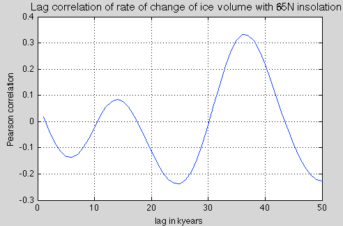
Figure 4
On the plus side, the first 200 kyrs look quite impressive, including terminations:

Figure 5
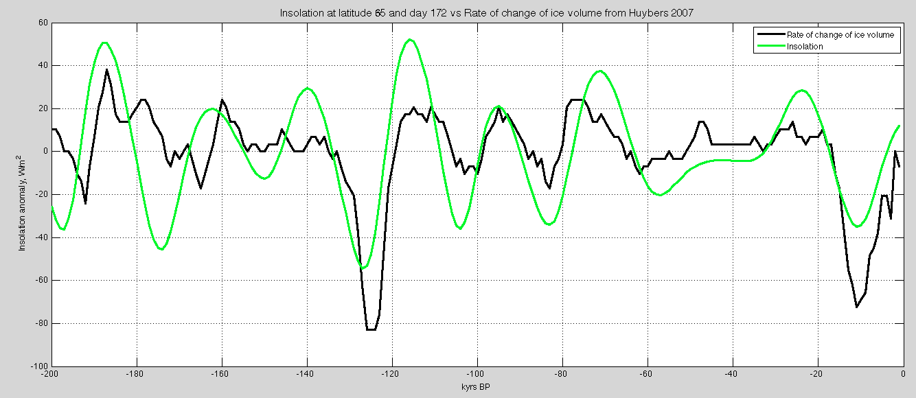
Figure 6
This has got me wondering.
What do we notice from the data for the first 200 kyrs (figure 6)? Well, the last two terminations (check out the last few posts) are easily identified because the rate of change of ice volume in proportion to insolation is about four times its value when no termination takes place.
Forgetting about the small problem of the Southern Hemisphere lead in the last deglaciation (Part Eleven – End of the Last Ice age), there is something interesting going on here. Almost like a theory that is just missing one easily identified link, one piece of the jigsaw puzzle that just needs to be fitted in, and the new Nature paper is waiting..
Onto some details.. it seems that T-II, if marked by the various radiometric dating values we saw Part Thirteen – Terminator II, would cause the 100k-200k values to move out of phase (the big black dip at about 125 kyrs would move about 15 kyrs to the left). So my next objective (see Sixteen – Roe vs Huybers II) is to set an age marker for Termination II from the radiometric dating values and “slide” the Huybers 2007 dataset to this and the current T1 dating. Also, the ice core proxies recorded in deep ocean cores must lag real ice volume changes by some period like say 1 – 3 kyrs (see note 1). This helps the Roe hypothesis because the black curves move to the left.
Let’s see what happens with these changes.
And hopefully, sharp-eyed readers are going to identify opportunities for improvement in this article, as well as the missing piece of the puzzle that will lead to the coveted Nature paper..
Articles in the Series
Part One – An introduction
Part Two – Lorenz – one point of view from the exceptional E.N. Lorenz
Part Three – Hays, Imbrie & Shackleton – how everyone got onto the Milankovitch theory
Part Four – Understanding Orbits, Seasons and Stuff – how the wobbles and movements of the earth’s orbit affect incoming solar radiation
Part Five – Obliquity & Precession Changes – and in a bit more detail
Part Six – “Hypotheses Abound” – lots of different theories that confusingly go by the same name
Part Seven – GCM I – early work with climate models to try and get “perennial snow cover” at high latitudes to start an ice age around 116,000 years ago
Part Seven and a Half – Mindmap – my mind map at that time, with many of the papers I have been reviewing and categorizing plus key extracts from those papers
Part Eight – GCM II – more recent work from the “noughties” – GCM results plus EMIC (earth models of intermediate complexity) again trying to produce perennial snow cover
Part Nine – GCM III – very recent work from 2012, a full GCM, with reduced spatial resolution and speeding up external forcings by a factors of 10, modeling the last 120 kyrs
Part Ten – GCM IV – very recent work from 2012, a high resolution GCM called CCSM4, producing glacial inception at 115 kyrs
Pop Quiz: End of An Ice Age – a chance for people to test their ideas about whether solar insolation is the factor that ended the last ice age
Eleven – End of the Last Ice age – latest data showing relationship between Southern Hemisphere temperatures, global temperatures and CO2
Twelve – GCM V – Ice Age Termination – very recent work from He et al 2013, using a high resolution GCM (CCSM3) to analyze the end of the last ice age and the complex link between Antarctic and Greenland
Thirteen – Terminator II – looking at the date of Termination II, the end of the penultimate ice age – and implications for the cause of Termination II
Fourteen – Concepts & HD Data – getting a conceptual feel for the impacts of obliquity and precession, and some ice age datasets in high resolution
Sixteen – Roe vs Huybers II – remapping a deep ocean core dataset and updating the previous article
Seventeen – Proxies under Water I – explaining the isotopic proxies and what they actually measure
Eighteen – “Probably Nonlinearity” of Unknown Origin – what is believed and what is put forward as evidence for the theory that ice age terminations were caused by orbital changes
Nineteen – Ice Sheet Models I – looking at the state of ice sheet models
References
In defense of Milankovitch, Gerard Roe, Geophysical Research Letters (2006) – free paper
Glacial variability over the last two million years: an extended depth-derived agemodel, continuous obliquity pacing, and the Pleistocene progression, Peter Huybers, Quaternary Science Reviews (2007) – free paper
How long to oceanic tracer and proxy equilibrium?, C Wunsch & P Heimbach, Quaternary Science Reviews (2008) – free paper
Datasets for Huybers 2007 are here:
ftp://ftp.ncdc.noaa.gov/pub/data/paleo/contributions_by_author/huybers2006/
and
http://www.people.fas.harvard.edu/~phuybers/Progression/
Insolation data calculated from Jonathan Levine’s MATLAB program (just ask for this data in Excel or MATLAB format)
Notes
Note 1: See, for example, Wunsch & Heimbach 2008:
The various time scales for distribution of tracers and proxies in the global ocean are critical to the interpretation of data from deep- sea cores. To obtain some basic physical insight into their behavior, a global ocean circulation model, forced to least-square consistency with modern data, is used to find lower bounds for the time taken by surface-injected passive tracers to reach equilibrium. Depending upon the geographical scope of the injection, major gradients exist, laterally, between the abyssal North Atlantic and North Pacific, and vertically over much of the ocean, persisting for periods longer than 2000 years and with magnitudes bearing little or no relation to radiocarbon ages. The relative vigor of the North Atlantic convective process means that tracer events originating far from that location at the sea surface will tend to display abyssal signatures there first, possibly leading to misinterpretation of the event location. Ice volume (glacio-eustatic) corrections to deep-sea d18O values, involving fresh water addition or subtraction, regionally at the sea surface, cannot be assumed to be close to instantaneous in the global ocean, and must be determined quantitatively by modelling the flow and by including numerous more complex dynamical interactions.


I have a few more crazy ideas.
It might not just be orbital changes. It seems very likely that there should be mechanical components, in concert with orbital changes, that ultimately leads to terminations.
Obviously, heavy glaciation dominates the Pleistocene punctuated by brief periods of melt-back. One conceptual model is that something builds up or breaks down over +/-100Kyears so that the next push causes a catastrophic failure of the ice sheets.
The dust build-up theory goes with that. The record indicates that glacial periods contain several minor melt-backs that might help accumulate dust near the ice sheet surface. I’m actually liking this less.
We know that isostatic rebound follows ice removal. Perhaps the ice sheets are weakened over time by the minor melt-offs (which are likely not uniformly distributed) causing local and regional crustal rebound that helps create fully penetrating fissures and faults within the sheets. After 100Kyears of this jacking up and down, a minor melt-off and crustal rebound causes enough structural failure, combined with dust buildup and the ice sheets fail completely.
Another idea is that the ice sheets eventually fail because at some local and regional areas, their weight exceeds the structural capacity of the ice sheet. One could imagine in areas like the great lakes and Hudson Bay where the ice sheets have deep roots, the roots might prevent some lateral movement and allow for a buildup of ice that does not induce enough lateral displacement and they come down like a house of cards.
Finally, perhaps the orbital features are somehow additive or cause the minor melt-offs. Then, when an orbital change occurs, perhaps not always insolation at 65N, that is enough to cause ice sheets, perhaps weakened over 100Kyears of an unsettled life, to fall into a cascading failure.
It’s OK. I have a state-issued license to wave my arms.
I can taste that Nature paper already!
Howard,
Not really crazy. The dust idea is a very interesting one.
Here is a bit more data to whet your appetite – from Millennial-scale variability during the last glacial: The ice core record, E.W. Wolff, J. Chappellaz, T. Blunier, S.O. Rasmussen, A. Svensson, Quaternary Science Reviews (2010):
Click to Expand
So this is not the glacial to interglacial transition, but instead the “within glacial” transitions.
Which might be the key.
Can anyone explain to me why everyone uses 65N to calculate insolation ? I realise that Milankovitch originally proposed this because it more or less corresponds to the Arctic Circle, but is there any other reason ? When insolation is high at the Arctic it is simultaneously low at the Antarctic for finite eccentricity. Higher eccentricity accentuates this north-south asymmetry.
Following Roe’s paper I calculated the maximum insolation at the North Pole and compared it with the differential ice volume using LR04. In this plot I invert the insolation to better show the correlation with ice volume, because higher insolation = lower ice volume. Correlation is better also from before 200,000 years ago:
However there is definitely a another physical cause for the 100,000 y cycle waiting to be discovered. My current pet theory is that the same planetary gravitational effects that perturb the earth’s orbit into a higher eccentricity must also change the moon’s effective orbit round the earth. This leads to amplified tides which help break down the ice sheets. When this coincides with enhanced insolation at northern latitudes an interglacial melt down is triggered.
Clive,
It’s just Milankovitch’s original theory.
Lots of people have proposed different values because nothing really fits all of the data (like 45N, spring at latitude blah, southern hemisphere insolation, Antarctica summer insolation when temperature is above value blah1, gradient of insolation between latitude blah2 and blah3).
Roe also looked for the best fit, as he made the point:
I thought about finding a best fit for the article but didn’t expect it to find anything of useful value. However, I will run a test..
Clive,
Here is the correlation at zero lag for every latitude and every day:
Click to expand
Same view rotated:
Click to expand
It’s clear – as you indicate – that 90’N summer (early Aug) is a correlation optimum, but so is 90’S summer.
I checked with a lag of 3,000 years, on the grounds that there must be some significant lag between ice sheet changes and the δ18O on the ocean floor being fixed by foraminifera.
The shape of the result looks the same (as the 3d view above) but the maximum correlation goes from 0.3 down to 0.24.
I don’t think these correlation values have much real meaning.
But for reference, here are the plots where zero lag correlation peaks from both polar regions:
Click to expand
A simple, parsimonious solution to the graphs in this article is that the Huybers dataset, based on a sedimentation model, drifts out of phase with reality, and the approach of orbital tuning is the correct one.
Food for thought
Or the sedimentation model needs more work. The fact that it appears to be a gradual phase shift rather than a complete loss of coherence is a fairly strong indication that the sedimentation only dating is off.
If the only indication that the times of the dataset are off is the orbital coherence then it doesn’t help with an improved solution. Given that the whole point of the dataset was to create one without assumptions about orbital tuning.
And we’re back to the fact that you couldn’t tune to the orbital signal unless it were actually present. Therefore any dating scheme that does not produce phase coherence is almost certainly flawed. The question is whether such a scheme could ever be produced without peeking.
Yes, actually looking at the plots, it is obvious that with some arbitrary phase drifts, you can get pretty good corelation. The shapes still look very similar, that is something. This could be resolved ofcourse only if someone can explain the drifts in the data without using orbital data. But I think it looks interestiing.
For interest, I ran the comparison with LR04 (which is tuned to insolation at 65’N).
The Pearson correlation for insolation at 65’N and LR04 over 500 kyrs = 0.29.
The correlation over 200 kyrs = 0.29.
Not a surprise to find the consistent correlation (see body of article), I was interested in what the value actually was for this tuned dataset.
[…] « Ghosts of Climates Past – Fifteen – Roe vs Huybers […]
This paper shows a quite remarkable correlation between dust deposits in EPICA ice cores and ice core temperature.
F.Lambert et al. Centennial mineral dust variability in high-resolution ice core data from Dome C, Antarctica. Clim.Past,8,609-623,2012
The solution to the underlying cause of interglacial warming must first explain why the observed increases in dust deposits preceded them.
Clive: Do you have a link to the full paper? From what I can tell, even intera-glacial temperature increases generally follow periods of dust spikes. Maybe there is more to dust than dirty glaciers. It looks like it can have huge effects on weather and weather has huge effects on dust. I think I smell hysteresis.
http://climatemodeling.science.energy.gov/research-highlights/desert-dust-intensifies-summer-rainfall-us-southwest
The dust increases precipitation by up to 40 percent during the summer rainy season in Arizona, New Mexico, and Texas. Their study, the first on the U.S. Southwest summer monsoon, found that the heat pump effect is consistent with how dust acts on West African and Asian monsoon regions. Understanding how dust contributes to atmospheric heating is important for predicting drought and rainfall patterns in this region and others in the world with rising populations.
Click to access Delmonte_2004a.pdf
…..suggest the dominant contribution to East Antarctic dust in glacial times deriving from the southern South American region of Patagonia and the
Pampas
Click to access feltonmasters.pdf
We have found evidence for relatively intense weathering and humid conditions…..60-50 ka BP. After 50 ka BP and until 32 ka….climate conditions became somewhat drier,…moderately humid. …. was followed by intense aridity with possible evidence for eolian dust deposition between 32-14 ka BP, during the same period of the Last Glacial Maximum. The paleoclimate record…Lake Tanganyika basin…Kalya horst
site…past 60 ka BP….striking similarities to the marine isotope…
glacial ice volume, and much less correspondence to precessionally driven insolation forcing over the same time interval.
Click to access DUSTSPEC_Lamomt_Miller_web.pdf
Conclusions
1 Dust aerosols influence climate by darkening bright surfaces•
2 Dust particles containing iron can increase photosynthesis within the ocean mixed layer, drawing down atmospheric CO2
3 Dust aerosols reduce mixing within the boundary layer, confining pollutants near the surface
4 Although soil dust aerosols are created by wind erosion of the driest environments, they affect precipitation because of downwind transport into wetter regions, and atmospheric dynamics that extends the influence of radiative heating beyond the dust layer.
5 Precipitation is reduced globally by dust radiative forcing at the surface, although precipitation can increase locally in regions of positive forcing.
6 Similarly, dust can increase cloud cover by driving a circulation that converges moisture.
7 Dust particles inhibit rainfall in warm (water) clouds, and the larger particles are efficient ice nuclei that increase precipitation of ice phase particles.
8 Measurements of deposition that resolve mineral content would be very useful
Sorry for long delay in replying .
You can download the full paper here
Click to access cp-8-609-2012.pdf
I got lost somewhere in other blog discussions !
Thanks Clive, that was a good read.
Clive:The solution to the underlying cause of interglacial warming must first explain why the observed increases in dust deposits preceded them. This was confusing to me, but the paper cleared it up, thanks for the link.
From what I see in the paper, dust/dust flux are high during glacial periods and climb up to a peak prior to either Dansgaard-Oeschger (DO) events and the end of the glacial period, then decline to low interglacial dust/dust flux levels ~4,000-years before Temp and CO2 reach interglacial levels.
They conclude that changes in ocean circulation may result in increased precipitation in the dust source areas causing the atmosphere to be washed of particulates and more vegetation grows to hold the dust down.
The question remains, why do the regional weather patterns shift? Is the dust flux a factor in the atmosphere as condensation nuclei and/or the ocean as fertilizers? Perhaps dust albedo on Continental glaciers reaches a tipping point, initiating melt and shifting the weather patterns.
The dust/temp/CO2 time relationship is set in the ice, unlike the uncertain time relationship with the astronomical changes insolation, precession, etc.
Howard,
Yes and no. The dust/temp relationship with time is solid. CO2 has problems because the bubbles may not seal for a very long time. During the depths of a glacial period, snow accumulation in central Antarctica is very slow. The gas age and the ice age may differ by thousands of years, with the gas age always younger than the surrounding ice. Once all the 14C decays in ~50,000 years, the gas age can only be estimated from the estimated rate of accumulation.
The gas age question is complicated and I expect to write more about it in a later article.
Fresh snow allows air to circulate. Eventually the snow compacts into ice and finally the structure locks the air in.
As DeWitt says, in Antarctica snow accumulation is very low which means the depth of air circulation before “close off” corresponds to many thousands of years. By contrast, in Greenland, the snow accumulation is much higher which means the same depth corresponds to a shorter time – and less age uncertainty.
There are a few approaches to determining gas age.
1. The ‘firn model’, which is based on how the crystalline structure changes with depth – this allows us to calculate the difference between age of ice and age of gas, so if the ice can be dated we can estimate the age of the gas.
Ice can be dated in a number of ways, not just from accumulation estimates (constraints from 10Be events, volcanic events..).
2. Synchronization of Greenland and Antarctica using CH4. We have better dating for Greenland ice for at least 50,000 years by counting layers (higher accumulation rates in Greenland makes this possible). And the gas-ice age difference is lower in Greenland as mentioned above.
CH4 is a well-mixed gas globally, is captured in both Greenland and Antarctica ice cores and has significant variability over the thousand year timescale – so we can match up Greenland and Antarctica gas age – at least during periods of significant CH4 change.
Unfortunately, the best Greenland ice core (NGRIP) only goes back 123,000 years because it all melted prior to this date.
3. δ18O(atm) – in many of the graphs produced in this series we have seen δ18O from the ice as a proxy for temperature when it snowed out – also we can measure δD from ice which works on the exact same basis.
We also have measurements of δ18O in the gas trapped in the ice – this is the isotope of oxygen in the air, rather than in the ice. It appears that there is a strong correlation of δ18O(atm) with insolation changes and this presents the opportunity to at least count precession cycles (ie we can ensure that older dates have accuracies constrained to at least +/- 10,000 years – half a precession cycle).
4. Novel methods, which I am just reading up on at the moment. These include N2/O2 ratios, volume of air trapped in the ice, fractionation of isotopes (like 15N) due to thermal and gravitational effects.
If anyone is interested in papers which explain any of these points, just ask.
Otherwise these points will all get covered in future articles along with references, and I will do a better job than the brief note above of explaining how all this fits together.
DeWitt and SOD, thanks for setting me straight on the gas problem in Antarctica. Looking forward to future posts. In no hurry, there is plenty to chew on as it is.
[…] Fifteen – Roe vs Huybers – reviewing In Defence of Milankovitch, by Gerard Roe […]
I just discovered this post; however, it may be worth a note about the SPECMAP tuning work done 35 years ago . It’s true the O18 curves were tuned to orbital parameters but the tuning was constrained by half a dozen or so C14 and/or microfossil extinction dates in the deep sea sediment cores used. Bioturbation, sediment rates, and sampling intervals are going to make exact dates a bit fuzzy of course, but IIRC the dating accuracy was estimated to be within 2-3kyrs.
Gary,
Can you give a reference or explain the 2-3 kyrs accuracy. Perhaps in the first 50 kyrs it might be that accurate, but not at say 500 kyrs.
[…] I’ll use the same temperature proxy dataset used in the discussion by Science of Doom here and here, which is the Huybers ∂18O dataset . For the insolation, I’m using the same Berger […]
[…] I’ll use the same temperature proxy dataset used in the discussion by Science of Doom here and here, which is the Huybers ∂18O dataset . For the insolation, I’m using the same Berger […]
We absolutely love your blog and find the majority of your post’s to be precisely what
I’m looking for. can you offer guest writers to
write content for yourself? I wouldn’t mind creating a post
or elaborating on many of the subjects you write about here.
Again, awesome website!