In Part Seven – GCM I through Part Ten – GCM IV we looked at GCM simulations of ice ages.
These were mostly attempts at “glacial inception”, that is, starting an ice age. But we also saw a simulation of the last 120 kyrs which attempted to model a complete ice age cycle including the last termination. As we saw, there were lots of limitations..
One condition for glacial inception, “perennial snow cover at high latitudes”, could be produced with a high-resolution coupled atmosphere-ocean GCM (AOGCM), but that model did suffer from the problem of having a cold bias at high latitudes.
The (reasonably accurate) simulation of a whole cycle including inception and termination came by virtue of having the internal feedbacks (ice sheet size & height and CO2 concentration) prescribed.
Just to be clear to new readers, these comments shouldn’t indicate that I’ve uncovered some secret that climate scientists are trying to hide, these points are all out in the open and usually highlighted by the authors of the papers.
In Part Nine – GCM III, one commenter highlighted a 2013 paper by Ayako Abe-Ouchi and co-workers, where the journal in question, Nature, had quite a marketing pitch on the paper. I made brief comment on it in a later article in response to another question, including that I had emailed the lead author asking a question about the modeling work (how was a 120 kyr cycle actually simulated?).
Most recently, in Eighteen – “Probably Nonlinearity” of Unknown Origin, another commented highlighted it, which rekindled my enthusiasm, and I went back and read the paper again. It turns out that my understanding of the paper had been wrong. It wasn’t really a GCM paper at all. It was an ice sheet paper.
There is a whole field of papers on ice sheet models deserving attention.
GCM review
Let’s review GCMs first of all to help us understand where ice sheet models fit in the hierarchy of climate simulations.
GCMs consist of a number of different modules coupled together. The first GCMs were mostly “atmospheric GCMs” = AGCMs, and either they had a “swamp ocean” = a mixed layer of fixed depth, or had prescribed ocean boundary conditions set from an ocean model or from an ocean reconstruction.
Less commonly, unless you worked just with oceans, there were ocean GCMs with prescribed atmospheric boundary conditions (prescribed heat and momentum flux from the atmosphere).
Then coupled atmosphere-ocean GCMs came along = AOGCMs. It was a while before these two parts matched up to the point where there was no “flux drift”, that is, no disappearing heat flux from one part of the model.
Why so difficult to get these two models working together? One important reason comes down to the time-scales involved, which result from the difference in heat capacity and momentum of the two parts of the climate system. The heat capacity and momentum of the ocean is much much higher than that of the atmosphere.
And when we add ice sheets models – ISMs – we have yet another time scale to consider.
- the atmosphere changes in days, weeks and months
- the ocean changes in years, decades and centuries
- the ice sheets changes in centuries, millennia and tens of millenia
This creates a problem for climate scientists who want to apply the fundamental equations of heat, mass & momentum conservation along with parameterizations for “stuff not well understood” and “stuff quite-well-understood but whose parameters are sub-grid”. To run a high resolution AOGCM for a 1,000 years simulation might consume 1 year of supercomputer time and the ice sheet has barely moved during that period.
Ice Sheet Models
Scientists who study ice sheets have a whole bunch of different questions. They want to understand how the ice sheets developed.
What makes them grow, shrink, move, slide, melt.. What parameters are important? What parameters are well understood? What research questions are most deserving of attention? And:
Does our understanding of ice sheet dynamics allow us to model the last glacial cycle?
To answer that question we need a model for ice sheet dynamics, and to that we need to apply some boundary conditions from some other “less interesting” models, like GCMs. As a result, there are a few approaches to setting the boundary conditions so we can do our interesting work of modeling ice sheets.
Before we look at that, let’s look at the dynamics of ice sheets themselves.
Ice Sheet Dynamics
First, in the theme of the last paper, Eighteen – “Probably Nonlinearity” of Unknown Origin, here is Marshall & Clark 2002:
The origin of the dominant 100-kyr ice-volume cycle in the absence of substantive radiation forcing remains one of the most vexing questions in climate dynamics
We can add that to the 34 papers reviewed in that previous article. This paper by Marshall & Clark is definitely a good quick read for people who want to understand ice sheets a little more.
Ice doesn’t conduct a lot of heat – it is a very good insulator. So the important things with ice sheets happen at the top and the bottom.
At the top, ice melts, and the water refreezes, runs off or evaporates. In combination, the loss is called ablation. Then we have precipitation that adds to the ice sheet. So the net effect determines what happens at the top of the ice sheet.
At the bottom, when the ice sheet is very thin, heat can be conducted through from the atmosphere to the base and make it melt – if the atmosphere is warm enough. As the ice sheet gets thicker, very little heat is conducted through. However, there are two important sources of heat for surface heating which results in “basal sliding”. One source is geothermal energy. This is around 0.1 W/m² which is very small unless we are dealing with an insulating material (like ice) and lots of time (like ice sheets). The other source is the shear stress in the ice sheet which can create a lot of heat via the mechanics of deformation.
Once the ice sheet is able to start sliding, the dynamics create a completely different result compared to an ice sheet “cold-pinned” to the rock underneath.
Some comments from Marshall and Clark:
Ice sheet deglaciation involves an amount of energy larger than that provided directly from high-latitude radiation forcing associated with orbital variations. Internal glaciologic, isostatic, and climatic feedbacks are thus essential to explain the deglaciation.
..Moreover, our results suggest that thermal enabling of basal flow does not occur in response to surface warming, which may explain why the timing of the Termination II occurred earlier than predicted by orbital forcing [Gallup et al., 2002].
Results suggest that basal temperature evolution plays an important role in setting the stage for glacial termination. To confirm this hypothesis, model studies need improved basal process physics to incorporate the glaciological mechanisms associated with ice sheet instability (surging, streaming flow).
..Our simulations suggest that a substantial fraction (60% to 80%) of the ice sheet was frozen to the bed for the first 75 kyr of the glacial cycle, thus strongly limiting basal flow. Subsequent doubling of the area of warm-based ice in response to ice sheet thickening and expansion and to the reduction in downward advection of cold ice may have enabled broad increases in geologically- and hydrologically-mediated fast ice flow during the last deglaciation.
Increased dynamical activity of the ice sheet would lead to net thinning of the ice sheet interior and the transport of large amounts of ice into regions of intense ablation both south of the ice sheet and at the marine margins (via calving). This has the potential to provide a strong positive feedback on deglaciation.
The timescale of basal temperature evolution is of the same order as the 100-kyr glacial cycle, suggesting that the establishment of warm-based ice over a large enough area of the ice sheet bed may have influenced the timing of deglaciation. Our results thus reinforce the notion that at a mature point in their life cycle, 100-kyr ice sheets become independent of orbital forcing and affect their own demise through internal feedbacks.
[Emphasis added]
In this article we will focus on a 2007 paper by Ayako Abe-Ouchi, T Segawa & Fuyuki Saito. This paper is essentially the same modeling approach used in Abe-Ouchi’s 2013 Nature paper.
The Ice Model
The ice sheet model has a time step of 2 years, with 1° grid from 30°N to the north pole, 1° longitude and 20 vertical levels.
Equations for the ice sheet include sliding velocity, ice sheet deformation, the heat transfer through the lithosphere, the bedrock elevation and the accumulation rate on the ice sheet.
Note, there is a reference that some of the model is based on work described in Sensitivity of Greenland ice sheet simulation to the numerical procedure employed for ice sheet dynamics, F Saito & A Abe-Ouchi, Ann. Glaciol., (2005) – but I don’t have access to this journal. (If anyone does, please email the paper to me at scienceofdoom – you know what goes here – gmail.com).
How did they calculate the accumulation on the ice sheet? There is an equation:
Acc=Aref×(1+dP)Ts
Ts is the surface temperature, dP is a measure of aridity and Aref is a reference value for accumulation. This is a highly parameterized method of calculating how much thicker or thinner the ice sheet is growing. The authors reference Marshall et al 2002 for this equation, and that paper is very instructive in how poorly understood ice sheet dynamics actually are.
Here is one part of the relevant section in Marshall et al 2002:
..For completeness here, note that we have also experimented with spatial precipitation patterns that are based on present-day distributions.
Under this treatment, local precipitation rates diminish exponentially with local atmospheric cooling, reflecting the increased aridity that can be expected under glacial conditions (Tarasov and Peltier, 1999).
Paleo-precipitation under this parameterization has the form:
P(λ,θ,t) = Pobs(λ,θ)(1+dp)ΔT(λ,θ,t) x exp[βp.max[hs(λ,θ,t)-ht,0]] (18)
The parameter dP in this equation represents the percentage of drying per 1C; Tarasov and Peltier (1999) choose a value of 3% per °C; dp = 0:03.
[Emphasis added, color added to highlight the relevant part of the equation]
So dp is a parameter that attempts to account for increasing aridity in colder glacial conditions, and in their 2002 paper Marshall et al describe it as 1 of 4 “free parameters” that are investigated to see what effect they have on ice sheet development around the LGM.
Abe-Ouchi and co-authors took a slightly different approach that certainly seems like an improvement over Marshall et al 2002:
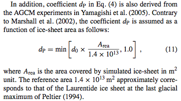
So their value of aridity is just a linear function of ice sheet area – from zero to a fixed value, rather than a fixed value no matter the ice sheet size.
How is Ts calculated? That comes, in a way, from the atmospheric GCM, but probably not in a way that readers might expect. So let’s have a look at the GCM then come back to this calculation of Ts.
Atmospheric GCM Simulations
There were three groups of atmospheric GCM simulations, with parameters selected to try and tease out which factors have the most impact.
Group One: high resolution GCM – 1.1º latitude and longitude and 20 atmospheric vertical levels with fixed sea surface temperature. So there is no ocean model, the ocean temperature are prescribed. Within this group, four experiments:
- A control experiment – modern day values
- LGM (last glacial maximum) conditions for CO2 (note 1) and orbital parameters with
- no ice
- LGM ice extent but zero thickness
- LGM ice extent and LGM thickness
So the idea is to compare results with and without the actual ice sheet so see how much impact orbital and CO2 values have vs the effect of the ice sheet itself – and then for the ice sheet to see whether the albedo or the elevation has the most impact. Why the elevation? Well, if an ice sheet is 1km thick then the surface temperature will be something like 6ºC colder. (Exactly how much colder is an interesting question because we don’t know what the lapse rate actually was). There will also be an effect on atmospheric circulation – you’ve stuck a “mountain range” in the path of wind so this changes the circulation.
Each of the four simulations was run for 11 or 13 years and the last 10 years’ results used:

From Abe-Ouchi et al 2007
Figure 1
It’s clear from this simulation that the full result (left graphic) is mostly caused by the ice sheet (right graphic) rather than CO2, orbital parameters and the SSTs (middle graphic). And the next figure in the paper shows the breakdown between the albedo effect and the height of the ice sheet:

From Abe-Ouchi et al 2007
Figure 2 – same color legend as figure 1
Now a lapse rate of 5K/km was used. What happens if the lapse rate of 9K/km was used instead? There were no simulations done with different lapse rates.
..Other lapse rates could be used which vary depending on the altitude or location, while a lapse rate larger than 7 K/km or smaller than 4 K/km is inconsistent with the overall feature. This is consistent with the finding of Krinner and Genthon (1999), who suggest a lapse rate of 5.5 K/km, but is in contrast with other studies which have conventionally used lapse rates of 8 K/km or 6.5 K/km to drive the ice sheet models..
Group Two – medium resolution GCM 2.8º latitude and longitude and 11 atmospheric vertical levels, with a “slab ocean” – this means the ocean is treated as one temperature through the depth of some fixed layer, like 50m. So it is allowing the ocean to be there as a heat sink/source responding to climate, but no heat transfer through to a deeper ocean.
There were five simulations in this group, one control (modern day everything) and four with CO2 & orbital parameters at the LGM:
- no ice sheet
- LGM ice extent, but flat
- 12 kyrs ago ice extent, but flat
- 12 kyrs ago ice extent and height
So this group takes a slightly more detailed look at ice sheet impact. Not surprisingly the simulation results give intermediate values for the ice sheet extent at 12 kyrs ago.
Group Three – medium resolution GCM as in group two, and ice sheets either at present day or LGM, with nine simulations covering different orbital values, different CO2 values of present day, 280 or 200 ppm.
There was also some discussion of the impact of different climate models. I found this fascinating because the difference between CCSM and the other models appears to be as great as the difference in figure 2 (above) which identifies the albedo effect as more significant than the lapse rate effect:
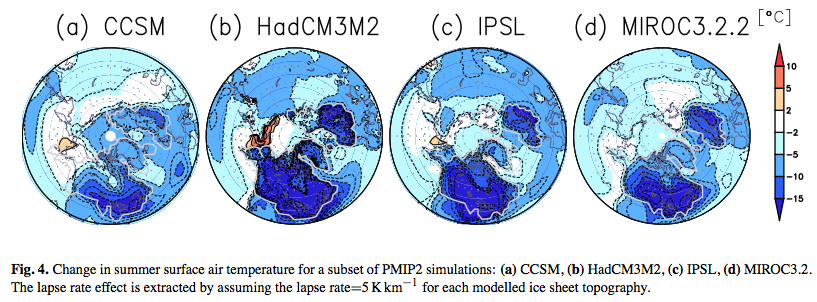
From Abe-Ouchi et al 2007
Figure 3
And this naturally has me wondering about how much significance to put on the GCM simulation results shown in the paper. The authors also comment:
Based on these GCM results we conclude there remains considerable uncertainty over the actual size of the albedo effect.
Given there is also uncertainty over the lapse rate that actually occurred, it seems there is considerable uncertainty over everything.
Now let’s return to the ice sheet model, because so far we haven’t seen any output from the ice sheet model.
GCM Inputs into the Ice Sheet Model
The equation which calculates the change in accumulation on the ice sheet used a fairly arbitrary parameter dp, with (1+dp) raised to the power of Ts.
The ice sheet model has a 2 year time step. The GCM results don’t provide Ts across the surface grid every 2 years, they are snapshots for certain conditions. The ice sheet model uses this calculation for Ts:
Ts = Tref + ΔTice + ΔTco2 + ΔTinsol + ΔTnonlinear
Tref is the reference temperature which is present day climatology. The other ΔT (change in temperature) values are basically a linear interpolation from two values of the GCM simulations. Here is the ΔTCo2 value:
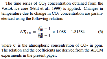
So think of it like this – we have found Ts at one value of CO2 higher and one value of CO2 lower from some snapshot GCM simulations. We plot a graph with Co2 on the x-axis and Ts on the y-axis with just two points on the graph from these two experiments and we draw a straight line between the two points.
To calculate Ts at say 50 kyrs ago we look up the CO2 value at 50 kyrs from ice core data, and read the value of TCO2 from the straight line on the graph.
Likewise for the other parameters. Here is ΔTinsol:
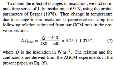
So the method is extremely basic. Of course the model needs something..
Now, given that we have inputs for accumulation on the ice sheet, the ice sheet model can run. Here are the results. The third graph (3) is the sea level from proxy results so is our best estimate of reality, with (4) providing model outputs for different parameters of d0 (“desertification” or aridity) and lapse rate, and (5) providing outputs for different parameters of albedo and lapse rate:
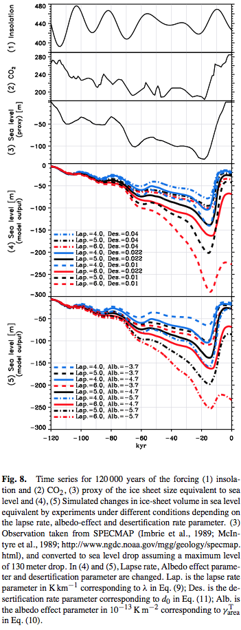
From Abe-Ouchi et al 2007
Figure 4
There are three main points of interest.
Firstly, small changes in the parameters cause huge changes in the final results. The idea of aridity over ice sheets as just linear function of ice sheet size is very questionable itself. The idea of a constant lapse rate is extremely questionable. Together, using values that appear realistic, we can model much less ice sheet growth (sea level drop) or many times greater ice sheet growth than actually occurred.
Secondly, notice that the time of maximum ice sheet (lowest sea level) for realistic results show sea level starting to rise around 12 kyrs, rather than the actual 18 kyrs. This might be due to the impact of orbital factors which were at quite a low level (i.e., high latitude summer insolation was at quite a low level) when the last ice age finished, but have quite an impact in the model. Of course, we have covered this “problem” in a few previous articles in this series. In the context of this model it might be that the impact of the southern hemisphere leading the globe out of the last ice age is completely missing.
Thirdly – while this might be clear to some people, but for many new to this kind of model it won’t be obvious – the inputs for the model are some limits of the actual history. The model doesn’t simulate the actual start and end of the last ice age “by itself”. We feed into the GCM model a few CO2 values. We feed into the GCM model a few ice sheet extent and heights that (as best as can be reconstructed) actually occurred. The GCM gives us some temperature values for these snapshot conditions.
In the case of this ice sheet model, every 2 years (each time step of the ice sheet model) we “look up” the actual value of ice sheet extent and atmospheric CO2 and we linearly interpolate the GCM output temperatures for the current year. And then we crudely parameterize these values into some accumulation rate on the ice sheet.
Conclusion
This is our first foray into ice sheet models. It should be clear that the results are interesting but we are at a very early stage in modeling ice sheets.
The problems are:
- the computational load required to run a GCM coupled with an ice sheet model over 120 kyrs is much too high, so it can’t be done
- the resulting tradeoff uses a few GCM snapshot values to feed linearly interpolated temperatures into a parameterized accumulation equation
- the effect of lapse rate on the results is extremely large and the actual value for lapse rate over ice sheets is very unlikely to be a constant and is also not known
- our understanding of ice sheet fundamental equations are still at an early stage, as readers can see by reviewing the first two papers below, especially the second one
Articles in this Series
Part One – An introduction
Part Two – Lorenz – one point of view from the exceptional E.N. Lorenz
Part Three – Hays, Imbrie & Shackleton – how everyone got onto the Milankovitch theory
Part Four – Understanding Orbits, Seasons and Stuff – how the wobbles and movements of the earth’s orbit affect incoming solar radiation
Part Five – Obliquity & Precession Changes – and in a bit more detail
Part Six – “Hypotheses Abound” – lots of different theories that confusingly go by the same name
Part Seven – GCM I – early work with climate models to try and get “perennial snow cover” at high latitudes to start an ice age around 116,000 years ago
Part Seven and a Half – Mindmap – my mind map at that time, with many of the papers I have been reviewing and categorizing plus key extracts from those papers
Part Eight – GCM II – more recent work from the “noughties” – GCM results plus EMIC (earth models of intermediate complexity) again trying to produce perennial snow cover
Part Nine – GCM III – very recent work from 2012, a full GCM, with reduced spatial resolution and speeding up external forcings by a factors of 10, modeling the last 120 kyrs
Part Ten – GCM IV – very recent work from 2012, a high resolution GCM called CCSM4, producing glacial inception at 115 kyrs
Pop Quiz: End of An Ice Age – a chance for people to test their ideas about whether solar insolation is the factor that ended the last ice age
Eleven – End of the Last Ice age – latest data showing relationship between Southern Hemisphere temperatures, global temperatures and CO2
Twelve – GCM V – Ice Age Termination – very recent work from He et al 2013, using a high resolution GCM (CCSM3) to analyze the end of the last ice age and the complex link between Antarctic and Greenland
Thirteen – Terminator II – looking at the date of Termination II, the end of the penultimate ice age – and implications for the cause of Termination II
Fourteen – Concepts & HD Data – getting a conceptual feel for the impacts of obliquity and precession, and some ice age datasets in high resolution
Fifteen – Roe vs Huybers – reviewing In Defence of Milankovitch, by Gerard Roe
Sixteen – Roe vs Huybers II – remapping a deep ocean core dataset and updating the previous article
Seventeen – Proxies under Water I – explaining the isotopic proxies and what they actually measure
Eighteen – “Probably Nonlinearity” of Unknown Origin – what is believed and what is put forward as evidence for the theory that ice age terminations were caused by orbital changes
References
Basal temperature evolution of North American ice sheets and implications for the 100-kyr cycle, SJ Marshall & PU Clark, GRL (2002) – free paper
North American Ice Sheet reconstructions at the Last Glacial Maximum, SJ Marshall, TS James, GKC Clarke, Quaternary Science Reviews (2002) – free paper
Climatic Conditions for modelling the Northern Hemisphere ice sheets throughout the ice age cycle, A Abe-Ouchi, T Segawa, and F Saito, Climate of the Past (2007) – free paper
Insolation-driven 100,000-year glacial cycles and hysteresis of ice-sheet volume, Ayako Abe-Ouchi, Fuyuki Saito, Kenji Kawamura, Maureen E. Raymo, Jun’ichi Okuno, Kunio Takahashi & Heinz Blatter, Nature (2013) – paywall paper
Notes
Note 1 – the value of CO2 used in these simulations was 200 ppm, while CO2 at the LGM was actually 180 ppm. Apparently this value of 200 ppm was used in a major inter-comparison project (the PMIP), but I don’t know the reason why. PMIP = Paleoclimate Modelling Intercomparison Project, Joussaume and Taylor, 1995.


“Curiouser and curiouser!”
(Alice’s Adventures in Wonderland)
Somehow that seems to be the appropriate response.
The dust data previously presented suggests that desertification increases and albedo decreases exponentially over ~40Kyrs up to the LGM.
Is anyone aware of geologic evidence of a 75Kyr period where most of the ice sheet is frozen static to the crust?
Is there any speculation why the maximum calculated post LGM sea level peaks out ~10 meters below the current level.
It seems to me that without better simulation of the effects of ocean circulation changes, it is impossible to know what is really driving the system.
DeWitt and Howard, this is an historical post that doesn’t say much about the present science. Howard, an awful lot of work has been done on the issues you identified.
Thanks for the post, SoD. ICYMI, this new paper seems like something you’ll want to cover in this series. Also, where a paper is paywalled as with the 2013 one but where a public copy is available, please link to the latter so people can better follow along.
While it’s certainly the case for the 2007 paper that “small changes in the parameters cause huge changes in the final results,” we should bear in mind that in the real world small changes in some of the parameterized factors led to head-long collapses.
Re the ice sheet models in general, it’s become pretty obvious from multiple studies published in the last year or so that they fall vastly (IMO) short of real-world ice sheet response. That renders questionable the use of ice sheet model results to establish an upper limit on current ice sheet response rates, but is it necessarily relevant for paleo time scales?
Possibly 200 v. 180 is a CO2e adjustment?
Thanks for the papers, Steve. Based on the CO2e Wiki page, I get 203ppmv CO2e @(180/365)*412, so I’m sure you are right. The extra 3ppmv is probably because the CH4 fraction is lower at the LGM absent anthro sources.
Steve,
There is a helpful online overview of PMIP by S Joussaume and KE Taylor.
I can’t access the citation by Abe-Ouchi: Joussaume, S. and Taylor, K.: Status of the paleoclimate model- ing intercomparison project (PMIP), in: WCRP-2, First Interna- tional AMIP Scientific Conference, 15–19 May 1995, Monterey, CA. Proceedings, Geneva, World Meteorological Organisation. World Climate Research Programme, 415–430, 1995 so I used that online (and later) overview.
As a side note it’s an interesting, short non-technical read, especially for people not familiar with many of the dilemmas faced by modeling people. Why did we set these conditions like this? Why didn’t we do that? What objectives did we have? What do the comparisons tell us? What is the value of any results?
There’s no mention of equivalent forcing. And the pre-industrial and current values match up. If it was equivalent forcing the current value would shoot quite higher due to the CH4 increases I think.
And looking up that reference: The ice record of greenhouse gases, Raynaud et al, Science (1993), it seems that the Vostok record has 190-200ppm and that was the accepted value at the time.
So probably Abe-Ouchi et al 2007 has selected a value of CO2 at the LGM that allows for better intercomparison results with other studies. Another dilemma for modeling people..
[…] 2014/04/14: TSoD: Ghosts of Climates Past – Nineteen – Ice Sheet Models I […]
The bathymetry of the Arctic Ocean shows that during LGM with sea levels 100m lower than present, ocean circulation essentially stopped except for a very small channel in the N.Atlantic. There is a good discussion of this at Chiefio
This could also be a possible cause of the polar oscillation effect, since expanding ice sheets over Antarctica (with precession) will reduce global sea levels and close the Bering Straights in the Arctic. This then leads to delayed cooling in the Arctic.
What breaks the cycle ?
I(We) propose that this is due to a strong increase in regular Tidal flushing of the Arctic coincident with the Milankovitch 100,000y eccentricity cycle. The reason for this increase in lunar tidal forces is because the moon is subject to the same solar system gravitational re-alignments that perturb the earth’s orbit. This must also change the eccentricity of the moon’s orbit around the earth because the bodies have different mass. The net result of increased ellipticity is that the distance of closest approach of the moon to the earth decreases and tidal forces increase rapidly as 1/R^3.
Clive,
I see two problems with this hypothesis. First, I can’t find any data on how the lunar orbit’s eccentricity varies with the Earth’s orbit eccentricity over the 100,000 year eccentricity cycle. Second, with sea level more than 100m below the current level and the edge of the North American continental ice cap at the LGM being far from the ocean, I don’t see a role for tides.
It’s distinctly possible that the lunar orbit is chaotic enough that it isn’t possible to calculate precisely over that time period. We know that it is chaotic or the rotation period of the Moon wouldn’t be phase locked to it’s orbital period. There does appear to be evidence from the laser ranging experiments that there is residual variation in the eccentricity that can’t be explained by current orbital models.
Thanks for the reply DeWitt,
You are correct that there is no data on the variation of the effective lunar orbit eccentricity around the earth. The seminal work on solar system dynamics has been done over decades by the French group at Observatoire de Paris. – Lasker et al. They quote huge errors on the moon’s orbital parameters for 1 million years ago. However we can still do some simple estimates.
The earth-moon are really a binary planet system in orbit round the sun. When the eccentricity of the moon’s orbit round the earth is modified by tidal forces of the sun on the moon and reach a maximum at the earth’s perihelion when the orbital axes are aligned. Currently the minimum distance between earth and moon centres is 360495km.
At the LGM the earth/moon’s eccentricity around the sun was increased to 0.02 so the perihelion distance of the earth/moon system was reduced leading to 20% larger solar tides. These tides acting on the moon’s orbit therefore increase the maximum lunar eccentricity and reduce the shortest distance of approach to the earth by 5%. Combing both the larger maximum lunar tide with the larger solar tide then we can estimate how large perihelion spring tides were 20,000 years ago. This shows that spring tides were then 30% greater than today.
So what ?
800,000 years ago there was a switch from 41,000 year cycle of glaciations to a 100,000 year cycle with interglacials coincident with maximum eccentricity. This seems to have happened because a gradual overall cooling trend exceeded a threshold for the the maximum inclination to melt back the increasingly larger northern ice sheets. Something else was needed to trigger the collapse of ice sheets by enhanced summer insolation.
You say:
During the LGM most of the Arctic was covered in sea ice as well. The Bering straights were closed and the only influx of warmer water would have been through a narrow deep passage connected to the North Atlantic. There is physical evidence from the sea bed that the ice was grounded at depths up to 1000m. So the arctic was essentially isolated from heat transport from warmer souther oceans.
I am suggesting that “Milankovitch” enhanced tides helped flush water under the arctic ice sheets to aid the melt back of the arctic ice. Once warmer water began to enter in the arctic summer, then the melt back could finally overcome the threshold needed for insolation and albedo feedback alone to trigger an interglacial. This also explains the sawtooth shape.
In addition tides also act on glaciers and help to calving the ice. In addition maximum tractional forces occur at the poles.
So I am proposing that “Milankovitch” tides may be the feather which finally breaks the camels back !
Clive,
Sorry, that’s still an assertion with no evidence. It may be probable, but that’s all I’ll give you.
As far as melting sea ice, it’s the wind driven currents near the surface, not at depth, that cause melting. Once the water flowing up from the south cools, it sinks to the bottom because the salinity is higher and has little interaction with the layers above. See here, for example.
It is more than just an assertion because I scale up the observed changes in lunar eccentricity every 206 days as the semi major-axis aligns with the sun. This change to eccentricity is known to be caused by changing solar tidal forces.
The real assertion is that such “Milankovitch” super tides are the trigger for the break-up of the northern ice-sheets. I agree this is rather speculative but it does at least have the advantage of explaining the 100,000 year mystery !
Thanks for the link. I read:
I agree that the statement melting “under the ice” is wrong. Perhaps be a better statement tides cause ‘lifting & shifting’ of the ice. A comment on WUWT from a guy in Alaska actually reported hearing the ice creak and groan during tidal flows.
If tides can trigger earthquakes then they likewise increase internal stresses within the large ice sheets aiding their breakup. see: “Métivier, L., de Viron, O., Conrad, C. P., Renault, S., Diament, M., & Patau, G., 2009. Evidence of Earthquake triggering by the solid Earth tides, Earth and Planet. Sc. Lett., 278, 370-375, doi: 10.1016/j.epsl.2008.12.024.”
Clive,
I noticed this article today, thought you might be interested in it.
The evolution of tides and tidal dissipation over the past 21,000 years
// Journal of Geophysical Research, Oceans
Abstract
The 120m sea-level drop during the Last Glacial Maximum (LGM; 18–22 kyr BP) had a profound impact on the global tides and lead to an increased tidal dissipation rate, especially in the North Atlantic. Here, we present new simulations of the evolution of the global tides from the LGM to present for the dominating diurnal and semidiurnal constituents. The simulations are undertaken in time slices spanning 500 to 1000 years. Due to uncertainties in the location of the grounding line of the Antarctic ice sheets during the last glacial, simulations are carried out for two different grounding line scenarios. Our results replicate previously reported enhancements in dissipation and amplitudes of the semidiurnal tide during LGM and subsequent deglaciation, and they provide a detailed picture of the large global changes in M2 tidal dynamics occurring over the deglaciation period. We show that Antarctic ice dynamics and the associated grounding line location have a large influence on global semidiurnal tides, whereas the diurnal tides mainly experience regional changes and are not impacted by grounding line shifts in Antarctica.
Marshall and Clark link may be down. Great post.
Ragnaar,
Thanks – I found a replacement link and updated the article.
It’s a very good paper. This series was great and I learned a lot.
Has anyone looked at the contribution of the Tibetan Plateau? That’s a rather large area at low latitude that was covered with ice during the last ice age. The albedo effect at the latitude of the Tibetan Plateau is about 4x the effect at high latitudes for the same area. According to Wikipedia, the isostatic rebound since the last glacial termination has been about 650m. Absent anthropogenic CO2 and LULC changes, would it have already been ice covered instead of having shrinking glaciers?
” Absent anthropogenic CO2 and LULC changes, would it have already been ice covered instead of having shrinking glaciers?”
I think it will only be a wild guess. But I would guess that it would not be a new ice cover. Glaciers around the world melted for 250 years before the clear increase of CO2. So it has been a “natural” process Who knows when this natural melting stopped? Has it stopped?
LULCC started when agriculture was invented about 8,000 years ago. The CO2 and methane from ice core data stopped decaying about then. Ruddimann’s hypothesis is that’s what stopped the normal temperature decay back to glacial conditions that happened in most of the recent glacial-interglacial-glacial transitions.
Thank you for the link. Let`s take Ruddimann with a grain of salt. Farmers changed climate 8000 years ago by increasing CO2, and monsoons cooled it down by reducing CO2 in Tibet. I think you should have a very stable level of CO2 to let such small changes have so great impact. I don`t think the CO2 budget and variation would allow that. Just a layman opinion.
LIA had an increase in glaciation, and probably some reduction of OHC. This was not in balance with sun radiation and atmospheric components, so glaciers began to melt at the end if LIA. Was it the Tibet platou that washed out CO2 at the end of the Medival Warm Period? And the farmers who brought it back?
Sure. Lots of people don’t accept Ruddimann’s hypothesis. It’s not exactly what you call the consensus view.
The ~10ppmv drop in Law Dome CO2 from about 1600 to 1800 can probably be explained as take up and release from the ocean as a function of solubility with temperature and probably doesn’t have much to do with either farmers or Tibet.
The monsoons on relatively unweathered rock represents a fairly steady sink for CO2, if you believe Raymo and Ruddiman, since the uplift of the Tibetan plateau. You get spikes in CO2 at glacial terminations that would then be drawn down slowly. But that isn’t what’s happening now.
The Vostok ice core data shows CO2 increasing from a minimum of 182ppmv at ~18,0000 yr BP (gas age), increasing to 264ppmv 11,000 yr BP, declining to a minimum of 255ppmv at 7,000 yr BP and then increasing to what we consider the pre-industrial level of 285ppmv at 2,000 yr BP. Something caused that. The main argument against Ruddimann is that his hypothesis isn’t necessary. Ruddimann begs to differ and Ockham’s Razor isn’t probative one way or the other.
The fluctuation of CO2 in Antarctica from 1600-1800, though, is pretty strong evidence, IMO, that the Little Ice Age was a global phenomenon and not limited to a small area in the Northern Hemisphere as some would have it.
[…] [1]https://scienceofdoom.com/2014/04/14/ghosts-of-climates-past-nineteen-ice-sheet-models-i/ […]