In Part Six we looked at some of the different theories that confusingly go by the same name. The “Milankovitch” theories.
The essence of these many theories – even though the changes in “tilt” of the earth’s axis and the time of closest approach to the sun don’t change the total annual solar energy incident on the climate, the changing distribution of energy causes massive climate change over thousands of years.
One of the “classic” hypotheses is increases in July insolation at 65ºN cause the ice sheets to melt. Or conversely, reductions in July insolation at 65ºN cause the ice sheets to grow.
The hypotheses described can sound quite convincing. Well, one at a time can sound quite convincing – when all of the “Milankovitch theories” are all lined up alongside each other they start to sound more like hopeful ideas.
In this article we will start to consider what GCMs can do in falsifying these theories. For some basics on GCMs, take a look at Models On – and Off – the Catwalk.
Many readers of this blog have varying degrees of suspicion about GCMs. But as regular commenter DeWitt Payne often says, “all models are wrong, but some are useful“, that is, none are perfect, but some can shed light on the climate mechanisms we want to understand.
In fact, GCMs are essential to understand many climate mechanisms and essential to understand the interaction between different parts of the climate system.
Digression – Ice Sheets and Positive Feedback
For beginners, a quick digression into ice sheets and positive feedback. Melting and forming of ice & snow is undisputably a positive feedback within the climate system.
Snow reflects around 60-90% of incident solar radiation. Water reflects less than 10% and most ground surfaces reflect less than 25%. If a region heats up sufficiently, ice and snow melt. Which means less solar radiation gets reflected, which means more radiation is absorbed, which means the region heats up some more. The effect “feeds itself”. It’s a positive feedback.
In the annual cycle it doesn’t lead to any kind of thermal runaway or a snowball earth because the solar radiation goes through a much bigger cycle.
Over much longer time periods it’s conceivable that (regional) melting of ice sheets leads to more (regional) solar radiation absorbed, causing more melting of ice sheets which leads to yet more melting. And the converse for growth of ice sheets. The reason it’s conceivable is because it’s just that same mechanism.
Digression over.
Why GCMs ?
The only alternative is to do the calculation in your head or on paper. Take a piece of paper, plot a graph of the incident radiation at all latitudes vs the time period we are interested in – say 150 kyrs ago through to 100 kyrs – now work out by year, decade or century, how much ice melts. Work out the new albedo for each region. Calculate the change in absorbed radiation. Calculate the regional temperature changes. Calculated the new heat transfer from low to high latitudes (lots of heat is exported from the equator to the poles via the atmosphere and the ocean) due to the latitudinal temperature gradient, the water vapor transported, and the rainfall and snowfall. Don’t forget to track ice melt at high latitudes and its impact on the Meridional Overturning Circulation (MOC) which drives a significant part of the heat transfer from the equator to poles. Step to the next year, decade or century and repeat.
How are those calculations coming along?
A GCM uses some fundamental physics equations like energy balance and mass balance. It uses a lot of parameterized equations to calculate things like heat transfer from the surface to the atmosphere dependent on the wind speed, cloud formation, momentum transfer from wind to ocean, etc. Whatever we have in a GCM is better than trying to do it on a sheet of paper (and in the end you will be using the same equations with much less spatial and time granularity).
If we are interested in the “classic” Milankovitch theory mentioned above we need to find out the impact of an increase of 50W/m² (over 10,000 years) in summer at 65ºN – see figure 1 in Ghosts of Climates Past – Part Five – Obliquity & Precession Changes. What effect does the simultaneous spring reduction at 65ºN have. Do these two effects cancel each other out? Is the summer increase more significant than the spring reduction?
How quickly does the circulation lessen the impact? The equator-pole export of heat is driven by the temperature difference – as with all heat transfer. So if the northern polar region is heating up due to ice melting, the ocean and atmospheric circulation will change and less heat will be driven to the poles. What effect does this have?
How quickly does an ice sheet melt and form? Can the increases and reductions in solar radiation absorbed explain the massive ice sheet growth and shrinking?
If the positive feedback is so strong how does an ice age terminate and how does it restart 10,000 years later?
We can only assess all of these with a general circulation model.
There is a problem though. A typical GCM run is a few decades or a century. We need a 10,000 – 50,000 year run with a GCM. So we need 500x the computing power – or we have to reduce the complexity of the model.
Alternatively we can run a model to equilibrium at a particular time in history to see what effect the historical parameters had on the changes we are interested in.
Early Work
Many readers of this blog are frequently mystified by my choosing “old work” to illuminate a topic. Why not pick the most up to date research?
Because the older papers usually explain the problem more clearly and give more detail on the approach to the problem.
The latest papers are written for researchers in the field and assume most of the preceding knowledge – that everyone in that field already has. A good example is the Myhre et al (1998) paper on the “logarithmic formula” for radiative forcing with increasing CO2, cited by the IPCC TAR in 2001. This paper has mystified so many bloggers. I have read many blog articles where the blog authors and commenters throw up their metaphorical hands at the lack of justification for the contents of this paper. However, it is not mystifying if you are familiar with the physics of radiative transfer and the papers from the 70’s through the 90’s calculating radiative imbalance as a result of more “greenhouse” gases.
It’s all about the context.
We’ll take a walk through a few decades of GCMs..
We’ll start with Rind, Peteet & Kukla (1989). They review the classic thinking on the problem:
Kukla et al. [1981] described how the orbital configurations seemed to match up with gross climate variations for the last 150 millennia or so. As a result of these and other geological studies, the consensus exists that orbital variations are responsible for initiating glacial and interglacial climatic regimes. The most obvious difference between these two regimes, the existence of subpolar continental ice sheets, appears related to solar insolation at northern hemisphere high latitudes in summer. For example, solar insolation at these latitudes in August and September was reduced, compared with today’s values, around 116,000 years before the present (116 kyr B.P.), during the time when ice growth apparently began, and it was increased around 10 kyr B.P. during a time of rapid ice sheet retreat [e.g., Berger, 1978] (Figure 1).
And the question of whether basic physics can link the supposed cause and effect:
Are the solar radiation variations themselves sufficient to produce or destroy the continental ice sheets?
The July solar radiation incident at 50ºN and 60ºN over the past 170 kyr is shown in Figure 1, along with August and September values at 50ºN (as shown by the example for July, values at the various latitudes of concern for ice age initiation all have similar insolation fluctuations). The peak variations are of the order of 10%, which if translated with an equal percentage into surface air temperature changes would be of the order of 30ºC. This would certainly be sufficient to allow snow to remain throughout the summer in extreme northern portions of North America, where July surface temperatures today are only about 10ºC above freezing.
However, the direct translation ignores all of the other features which influence surface air temperature during summer, such as cloud cover and albedo variations, long wave radiation, surface flux effects, and advection.
[Emphasis added].
Various energy balance climate models have been used to assess how much cooling would be associated with changed orbital parameters. As the initiation of ice growth will alter the surface albedo and provide feedback to the climate change, the models also have to include crude estimates of how ice cover will change with climate. With the proper tuning of parameters, some of which is justified on observational grounds, the models can be made to simulate the gross glacial/interglacial climate changes.
However, these models do not calculate from first principles all the various influences on surface air temperature noted above, nor do they contain a hydrologic cycle which would allow snow cover to be generated or increase. The actual processes associated with allowing snow cover to remain through the summer will involve complex hydrologic and thermal influences, for which simple models can only provide gross approximations.
They comment then on the practical problems of using GCMs for 10 kyr runs that we noted above. The problem is worked around by using prescribed values for certain parameters and by using a coarse grid – 8° x 10° and 9 vertical layers.
The various GCMs runs are typical of the approach to using GCMs to “figure stuff out” – try different runs with different things changed to see what variations have the most impact and what variations, if any, result in the most realistic answers:
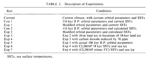
We have thus used the Goddard Institute for Space Studies (GISS) GCM for a series of experiments in which orbital parameters, atmospheric composition, and sea surface temperatures are changed. We examine how the various influences affect snow cover and low-elevation ice sheets in regions of the northern hemisphere where ice existed at the Last Glacial Maximum (LGM). As we show, the GCM is generally incapable of simulating the beginnings of ice sheet growth, or of maintaining low-elevation ice sheets, regardless of the orbital parameters or sea surface temperatures used.
[Emphasis added].
And the result:
The experiments indicate there is a wide discrepancy between the model’s response to Milankovitch perturbations and the geophysical evidence of ice sheet initiation. As the model failed to grow or sustain low-altitude ice during the time of high-latitude maximum solar radiation reduction (120-110 kyrB.P.), it is unlikely it could have done so at any other time within the last several hundred thousand years.
If the model results are correct, it indicates that the growth of ice occurred in an extremely ablative environment, and thus demanded some complicated strategy, or else some other climate forcing occurred in addition to the orbital variation influence (and CO2 reduction), which would imply we do not really understand the cause of the ice ages and the Milankovitch connection. If the model is not nearly sensitive enough to climate forcing, it could have implications for projections of future climate change.
[Emphasis added].
The basic model experiment on the ability of Milankovitch variations by themselves to generate ice sheets in a GCM, experiment 2, shows that in the GISS GCM even exaggerated summer radiation deficits are not sufficient. If widespread ice sheets at 10-m elevation are inserted, CO2 reduced by 70ppm, sea ice increases to full ice age conditions, and sea surface temperatures reduced to CLIMAP 18 kyr BP estimates or below, the model is just barely able keep these ice sheets from melting in restricted regions. How likely are these results to represent the actual state of affairs?
That was 1989 GCM’s.
Phillipps & Held (1994) had basically the same problem. This is the famous Isaac Held, who has written extensively on climate dynamics, water vapor feedback, GCMs and runs an excellent blog that is well-worth reading.
While paleoclimatic records provide considerable evidence in support of the astronomical, or Milankovitch, theory of the ice ages (Hays et al. 1976), the mechanisms by which the orbital changes influence the climate are still poorly understood..
..For this study we utilize the atmosphere-mixed layer ocean model.. In examining this model’s sensitivity to different orbital parameter combinations, we have compared three numerical experiments.
They describe the comparison models:
Our starting point was to choose the two experiments that are likely to generate the largest differences in climate, given the range of the parameter variations computed to have occurred over the past few hundred thousand years. The eccentricity is set equal to 0.04 in both cases. This is considerably larger than the present value of 0.016 but comparable to that which existed from ~90 to 150k BP.
In the first experiment, the perihelion is located at NH summer solstice and the obliquity is set at the high value of 24°.
In the second case, perihelion is at NH winter solstice and the obliquity equals 22°.
The perihelion and obliquity are both favorable for warm northern summers in the first case, and for cool northern summers in the second. These experiments are referred to as WS and CS respectively.
We then performed another calculation to determine how much of the difference between these two integrations is due to the perihelion shift and how much to the change in obliquity. This third model has perihelion at summer solstice, but a low value (22°) of the obliquity. The eccentricity is still set at 0.04. This experiment is referred to as WS22.
Sadly:
We find that the favorable orbital configuration is far from being able to maintain snow cover throughout the summer anywhere in North America..
..Despite the large temperature changes on land the CS experiment does not generate any new regions of permanent snow cover over the NH. All snow cover melts away completely in the summer. Thus, the model as presently constituted is unable to initiate the growth of ice sheets from orbital perturbations alone. This is consistent with the results of Rind with a GCM (Rind et al. 1989)..
In the next article we will look at more favorable results in the 2000’s.
Articles in the Series
Part One – An introduction
Part Two – Lorenz – one point of view from the exceptional E.N. Lorenz
Part Three – Hays, Imbrie & Shackleton – how everyone got onto the Milankovitch theory
Part Four – Understanding Orbits, Seasons and Stuff – how the wobbles and movements of the earth’s orbit affect incoming solar radiation
Part Five – Obliquity & Precession Changes – and in a bit more detail
Part Six – “Hypotheses Abound” – lots of different theories that confusingly go by the same name
Part Seven and a Half – Mindmap – my mind map at that time, with many of the papers I have been reviewing and categorizing plus key extracts from those papers
Part Eight – GCM II – more recent work from the “noughties” – GCM results plus EMIC (earth models of intermediate complexity) again trying to produce perennial snow cover
Part Nine – GCM III – very recent work from 2012, a full GCM, with reduced spatial resolution and speeding up external forcings by a factors of 10, modeling the last 120 kyrs
Part Ten – GCM IV – very recent work from 2012, a high resolution GCM called CCSM4, producing glacial inception at 115 kyrs
Pop Quiz: End of An Ice Age – a chance for people to test their ideas about whether solar insolation is the factor that ended the last ice age
Eleven – End of the Last Ice age – latest data showing relationship between Southern Hemisphere temperatures, global temperatures and CO2
Twelve – GCM V – Ice Age Termination – very recent work from He et al 2013, using a high resolution GCM (CCSM3) to analyze the end of the last ice age and the complex link between Antarctic and Greenland
Thirteen – Terminator II – looking at the date of Termination II, the end of the penultimate ice age – and implications for the cause of Termination II
Fourteen – Concepts & HD Data – getting a conceptual feel for the impacts of obliquity and precession, and some ice age datasets in high resolution
Fifteen – Roe vs Huybers – reviewing In Defence of Milankovitch, by Gerard Roe
Sixteen – Roe vs Huybers II – remapping a deep ocean core dataset and updating the previous article
Seventeen – Proxies under Water I – explaining the isotopic proxies and what they actually measure
Eighteen – “Probably Nonlinearity” of Unknown Origin – what is believed and what is put forward as evidence for the theory that ice age terminations were caused by orbital changes
Nineteen – Ice Sheet Models I – looking at the state of ice sheet models
References
Can Milankovitch Orbital Variations Initiate the Growth of Ice Sheets in a General Circulation Model?, Rind, Peteet & Kukla, JGR (1989) – behind a paywall, email me if you want to read it, scienceofdoom – you know what goes here – gmail.com
Response to Orbital Perturbations in an Atmospheric Model Coupled to a Slab Ocean, Phillipps & Held, Journal of Climate (1994) – free paper
New estimates of radiative forcing due to well-mixed greenhouse gases, Myhre et al, GRL (1998)


The phrase “essentially, all models are wrong, but some are useful” is from the famous statistician George E.P.Box.
So how does one distinguish a useful model from one that is wrong? An appropriate corollary to Box’s saying might be: “All models are wrong until PROVEN useful.”
I leave the philosophical and linguistic questions, and comment on usefulness in practice.
When a model is built the modeler expects it to answer questions of some specific type. When a large complex system is modeled a great deal of aggregation and simplification is needed. Model variables are mostly not identical to variables of the real system even when the same name is used for both variables.
A typical deviation is that normal averages are determined from empirical data to describe the real system, but the related variable of the model is a property of a large aggregate. Complex systems are nonlinear and that may make the property of the aggregate significantly different from the average of the real system.
The above is just one example of the more general phenomenon that an outsider is likely to misunderstand severely the model results, when they are given to him without extensive explanations, models are wrong in that sense. Most models of complex systems are directly useful only to people who work with those particular models extensively themselves. Only through that direct involvement can they build sufficient understanding on what the model is likely to represent correctly and what not. Models are learning tools for scientists.
Models are also means of communication among scientists who work with very similar models. In that the have a similar role as mathematical formulas, because they express precisely, what they do and what data they use as input. Various model intercomparison projects have taken advantage of the role of models as means of communication.
Pekka: I meant “All models are wrong until proven useful” as a PRAGMATIC restatement of Box’s saying, not a “philosophical or linguistic question”. WIth any model – which by Box’s generally-accepted saying is wrong – the first step must be assessing whether it is useful. You may remember Judith Curry’s discussions of “fitness for purpose”. You may also remember the paper she cited by Lorentz on the requirements for using climate models for detection and attribution of warming – the model must be constructed without using knowledge of earlier climate change.
In addition to their other limitations, GCMs contain about two dozen parameters whose precise values have not been established by controlled laboratory experiments. These parameters can be optimized one at a time for the IPCCs complicated models, but a set of parameters representing a global optimum for reproducing today’s climate is beyond our computing capabilities. Experiments with simpler models show that a optimum set of parameters can’t be identified and that the parameters used have a major impact on the model’s climate sensitivity. Multiple runs from any one climate model used by the IPCC don’t include the influence “parameter uncertainty” and therefore don’t project the full range of future climate that is compatible with our knowledge.
Frank,
Very many models are useful to some extent, but far fewer are known to have predictive skill in a well defined way. GCM type models are used all the time to test various ideas. An otherwise rather poor model may be very useful in that, if the model contains correctly that part of physics on which the idea is built as it can tell, whether other phenomena included in the model destroy the idea. This kind of work is typical use for the models.
When the purpose is to predict future climate in an emission (or forcing) scenario, the requirements are different. I’m confident that no large climate model has been developed or will be developed without any implicit tuning based on knowledge of climate history. In this case the statement of Lorenz should be interpreted to tell that statistical tests of the predictive power of the model cannot be properly done based on backcasting historical data. Success in backcasting does add trust in the predictive skill, but not in a quantifiable way, because the extent to which that is based on implicit tuning cannot be known.
By implicit tuning I mean all decisions made in building the model based on what the scientists have learned working with other models using historical data, or what they have learned from other scientists who have done the earlier work.
We know that the models contain parametrizations of phenomena that cannot be modeled from first principles. Every parametrization is an example of use of such information that makes it impossible to do proper statistical tests with historical data, unless the data is genuinely new for science and not just on improvement on earlier data or in some way correlated with earlier data.
Another problem is that there is not detailed and accurate enough data at all over a period long enough for testing the long term behavior of the models. Thus it’s possible to study, how well the models describe present climate and variability over short periods, but over longer periods the only things that can really be tested are, whether the model is behaving well enough to produce any predictions, and if that’s the case whether the predictions that it makes are not obviously wrong.
Pekka wrote: “I’m confident that no large climate model has been developed or will be developed without any implicit tuning based on knowledge of climate history.” Unfortunately climate history presumably includes both forced and natural variation. When you use a model for detection and attribution, you are asking the model to distinguish between natural and forced variation. When you tune your model using climate history, you are tuning the model to fit whatever natural variation is present in the climate history – the 1940’s warming and 1960’s cooling for example. A recent paper attributed the recent pause in warming to unusual coolness in the eastern equatorial Pacific (natural variation) and the 1975-1995 rapid warming to unusual warmth in the same region (also natural variation). Any model tuned to fit the rapid warming in 1975-1995 will be running too hot.
IMO (and I think Lorentz’s), to avoid fitting bias, you MUST tune your model to produce the best fit to PRESENT climate and then see what the model says about detection and attribution of change in the historical record. There are many aspects of present climate that can be fit: temperature, precipitation, TOA LWR and SWR, seasonal changes, latitudinal gradients, ARGO data, etc. Stainforth and colleagues investigated this approach with simplified models, but failed to find an optimum set of parameters.
Frank,
I agree on what you wrote. One should, however, not draw absolute conclusions based on pure principles like those that list the requirements for proper statistical testing.
It’s common for essentially all observational sciences (as distinct from sciences based on repeatable experiments) that satisfying fully the requirements of orthodox statistical testing are not fully satisfied, and that it’s furthermore impossible to determine, how badly they are broken. That by itself does not make drawing valid conclusions impossible, only making objective estimates of confidence ranges is impossible. That’s the way I interpret also Lorentz’s statement even if it’s formulated differently.
Extensive experience in working with models does help in estimating the accuracy and reliability of those features of the models that determine their suitability for making predictions, but this is an area, where many scientists do certainly err. Some of them are too willing to accept the model predictions, when they do not contradict their prejudices, while some others take an unnecessarily cautious view and consider the models virtually worthless as tools of prediction. To judge whom we should trust, we should at least learn in detail, how they justify their conclusions for themselves.
From scientists who trust in the validity of models, we should learn how extensively they have considered all known caveats, and how they have reached their conclusion that the predictions are not highly dependent on such details of the model, which have not been tested and for which alternatives are plausible. They should also tell, why the known failures of the models are not significant for the particular conclusions.
Concerning scientists who consider the models worthless for making predictions, we should learn, whether they know and understand the arguments of the other side, and why they regard the best sets of arguments unconvincing.
As far as I know it’s not possible to find open debate along the lines described above. There are several papers that take a critical look on models and present steps in that direction, but separate papers are not enough, we would need debate, where each side defends openly its views. Climate modeling is not the only field of science, where such debate is difficult to find, but the political controversy seems to make many even more wary of participating openly in such debate in spite of the fact that the political controversy does actually make an open debate only more important.
Pekka wrote: “It’s common for essentially all observational sciences … the requirements of orthodox statistical testing are not fully satisfied, and that it’s furthermore impossible to determine, how badly they are broken. That by itself does not make drawing valid conclusions impossible, only making objective estimates of confidence ranges is impossible”. By abandoning objective estimates of confidence ranges, aren’t you turning climate science into “climate opinion”. Can you cite other types of observational science where your generalization applies?
In his article “Chaos, Spontaneous Climatic Variation and Detection of the Greenhouse Effect”, Lorenz explained how detection and attribution should have been done. I don’t see where he advocates abandoning orthodox statistical methods. He clearly explains that our limited understanding of persistence of decadal temperature variation prevents us from using purely statistical methods to rejected the null hypothesis (that recent warming is due to natural variation). He then endorses using statistical methods to determine if the observed warming is statistically different from projections made by GCMs. However, he insists that the GCM method is “quite unacceptable” if the GCM has been tuned to fit the observed climate history. http://eaps4.mit.edu/research/Lorenz/Chaos_spontaneous_greenhouse_1991.pdf
As best I can tell, confidence intervals that take into account parameter uncertainty are so wide that the output useless for policymakers. Stainforth found warming from 2XCO2 ranging from 1.5 to 11 degK by varying 6 of about 20 parameters with an ensemble of simplified models. In the case of model output, appropriate confidence intervals are (IMO) a political, not scientific, problem. Policymakers expect increasingly accurate projections from all of the funds they have invested, but science doesn’t progress in direct proportion to funds expended. (See NIxon’s “War on Cancer” and Carter’s “Energy Independence”.)
Frank,
I can’t argue with your objections to the use of climate models in the PR war.
And I’ve been reading some of Koutsoyiannis’ papers recently – in between ice age GCM papers. I expect this series will run into some of his ideas so we’ll look at them in more detail soon, but he does an interesting assessment of statistical significance under AR1 vs Hurst-Kolmogorov and it’s quite fascinating. Some logarithmic relationships rather than linear or quadratic..
The subject of non-linearity is something that everyone in climate physics apparently signs up to – “hands up all those who believe that climate is non-linear”, gets all professional hands up.
But it seems that practical belief in this fundamental mechanism is clearly not at all prevalent.
Frank,
What was not possible in 1991 might well be possible now. Only the principle has remained the same, and on that the more detailed quote of Lorenz agrees with what I think.
It’s also quite possible that Stainforth errs to the direction of too little trust in the models. What I was asking for is an open debate between people with views like his and those with more trust in the predictive power of models.
I have also my doubts on overemphasis of arguments like those of Kotsoyiannis. How much predictive skill climate models have is a matter of judgment that should take into account all related information, and which cannot be done properly emphasizing any single method. Therefore a wider debate is needed, and many active modelers should participate in that together with people who understand potential problems of modeling from a different background.
It’s easy to list reasons why climate models “must” fail, much more difficult to tell, how severely they fail – or how much skill they after all have.
SOD: Thanks for the comment. I haven’t read much about Koutsoyiannis’ work, but I have followed the debate between Doug Keenan and the Met Office on the BIshop Hill blog. The debate and Lorenz 1991 clarified for me the critical difference between statistical models and physical models. Here are a few links if you haven’t followed this public debate:
Click to access AR5stat.pdf
http://metofficenews.wordpress.com/tag/doug-keenan/
Lorenz 1991 tells us that warming can’t be detected by purely statistical methods because we don’t have enough data to define the persistence of variations in decadal temperature. (When making this statement, he was discussing the situation that would exist if the rapid warming of the 1980’s persisted through the 1990’s. Since warming has been negligible since 2000, he was talking about today’s situation.) In response to Keenan, Met Office has also admitted that significant warming can’t be demonstrated by purely statistical methods. So detection and attribution of GHG-mediated warming depends on physical models (AOGCM’s), not the statistical models Keenan complains about. Lorenz 1991 endorses physical models, but only if the AOGCMs haven’t been “tuned” to match the historical record. The IPCCs models fail this test: they invariably pair high climate sensitivity with high sensitivity to aerosol and low climate sensitivity with low sensitivity to aerosols. If the models hadn’t been tuned to fit the historical record, parameter uncertainty probably would prevent AOGCMs from successfully attributing warming to GHGs.
It seems to me that Keenan’s efforts are misdirected because physical sciences rarely rely upon purely statistical models to analyze data. This was best illustrated to me when my son brought home some data from math class showing how many pennies could be placed in a cup suspended from a “bridge” made of dry spaghetti strands before the bridge would break. The number of stands of spaghetti and the span of the bridge were varied. (The purpose of the “experiment” was to introduce functions of more than one variable, not uncover the laws of physics, but I wanted to show my son how such data could be used to discover new laws. Best of all, I didn’t know the answer to the question we had encountered by accident!) It was easy to show that n strands could carry n times the load. The data from varying the span couldn’t choose between an inverse or inverse-square relationship and an exponent of -1.3 for a power law wasn’t very satisfying either. Quadratics and negative exponentials also looked possible. Given the physical limitations of the system, it was impossible to carry out experiments with short or long enough bridges to distinguish between all of these possibilities. My teaching experience was a failure because I forget that we never prove that scientific theories (models) are correct; we eliminate theories (models) that are inconsistent with observations. It turns out that the carrying capacity of a bridge fits a lever arm model (force time distance yielding an inverse law) and eventually we made some sense out of the data. Without a physical model (a hypothesis), the data could have been fit by infinitely many mathematical models.
It seems to me that Keenan is as lost in statistical models for global temperature as I was lost in mathematical equations that could be fit to our bridge capacity data. I’ll be interested your post on in Koutsoyiannis’ work, but I suspect the critical science is being done with physical models (AOGCMs), not the statistical models.
(If I understand the situation correctly, the stock market fits a random-walk model. That doesn’t mean that price-to-earnings ratio has nothing to do with the behavior of the stock market.)
Pekka: If you look carefully at Lorenz 1991, you see that he is discussing the detection and attribution problem that would exist in 2000 (after 2 decades of warming) assuming the 1990’s saw the same warming as the 1980’s. Given the lack of warming in the last decade, this is roughly the situation we face today.
When you speak of Stainforth “[erring in] the direction of too little trust in the models” and later of “judgment, you are again speaking of “climate opinion” not climate science. I personally don’t know (or care) how much Stainforth “trusts” climate models – the important thing is the data: He demonstrated that simultaneous random variation of six parameters (within established limits) in his models changed climate sensitivity by a factor of 7 without degrading the model’s performance at reproducing current climate. Then he tried and failed to find some subset of the tested range for any parameter that consistently produced an inferior representation of current climate. (This assumes that I correctly understood his work.)
The issue isn’t whether climate models “fail” or not; if the current pause continues, they will almost certainly be “re-tuned” so that observed and projected warming barely agree within uncertainly limits. The enhanced greenhouse effect from anthropogenic GHGs IS warming the planet – whether or not we can currently “prove” that “most” of the current warming is anthropogenic or natural variation. If we can prove using climate models that the current observed warming is unlikely to represent natural variation, then there is a clear scientific need to search of an explanation for that warming. However, the CONVERSE isn’t true: Even if we can’t rule out natural variation, the warming could be anthropogenic. Physics predicts that SOME of the warming will be anthropogenic; but ALL of the warming could be anthropogenic, or MORE THAN ALL of the warming could be anthropogenic (with some negated by natural variation). The desire to claim that MOST of the warming is anthropogenic is motivated by politics – and certainly not our confidence in our understanding of natural variability.
The real issue IS what range of climate sensitivity is found in all possible climate models that reproduce current climate with reasonable accuracy. Historical climate change is irrelevant, because we don’t know how much of that change is due to natural variation. Exaggerating our ability to model natural variability has led to disaster with the current pause in warming and semi-plausible charges that AGW is a hoax.
Frank,
First of all my impression is that relatively straightforward estimates of transient climate response (TCR) from instrumental data with some support of climate models is presently the best way of determining climate sensitivity over periods most significant for decision-making. A few years ago climate models had a more significant role and at the time UNFCCC and IPCC were created models were the only way. Paleoclimatic studies are one more source, but I have many reservations on their use due to the unknown dependency on the narratives needed in their interpretation.
Each of model based studies tells some specific information of limited generalizability, so does also Stainforth et al. I have often used the expression that we have quite a lot of information on behavior of climate, but the information is sparse. By sparse I mean that the various pieces are not strongly interconnected in the way that we would have solid precise knowledge on any major part of the whole issue. Therefore little can be concluded by purely objective methods. The total amount of information is, however, large and sets many constraints on the picture (or ultimate model) we have on the behavior of the Earth system. Stainforth et al observe that one specific model may be varied to give very different results, but does not tell, whether some further well justified constraints would have prevented that.
You write that you are not interested about “climate opinion”. What I have tried to say is that a very sizable fraction of good science is in part subjective, it’s about “opinions”. Disallowing opinions would be destructive for the success of science. We mus learn to live with science dependent on opinions, but that means also that scientists must learn to be very careful in forming their opinions. The community of scientists of each field must cooperate on getting rid of unsupportable conclusions. That requires open debate where all arguments are taken by their merit. The resulting conclusions are still uncertain at a level impossible to judge precisely, but that’s the best science can produce. It’s important that the process is not biased either towards belittling uncertainties nor towards exaggerating them.
I’m sure that some climate modelers do not satisfy the requirement of being very careful in forming their opinions, while some others fare better. I’m afraid that the debate has not been open enough and unbiased enough. Results like those of Stainforth et al are input to the debate as are numerous other scientific papers, and the understanding individuals have learned in using models and studying climate by other means.
Frank,
One more comment.
We are not in the same situation we were in 2000. One full decade without returning back to earlier temperatures is very significant. It adds very much to the power of the observational evidence, and is important for my conclusion that the instrumental data has taken over as the best source on climate sensitivity (as measured by TCR).
Pekka,
There are problems with measuring climate sensitivity.
One is described in the series Measuring Climate Sensitivity – Part One, which involves some “contamination” issues, originally raised by Spencer.
The other is that certain phases of climate have their own pattern on their own timescale.
For example, El Nino has a pattern that involves positive feedback and then the system dies away. That has a life of a few years. Over what period do you measure the climate sensitivity? Do you measure it over multiple El Ninos, or over one?
Other climate modes have periods that we think we know and many more are yet to be discovered. Any mode that has a period larger than we expect will not result in the climate sensitivity being measured correctly.
This raises the issue that climate sensitivity cannot be measured in the absence of a model. And what is the model? Well, we are trying to measure climate sensitivity without reference to the model. Maybe that is the problem.
I’m not sure I have understood this aspect of climate measurement.
I think it is an important calculation to attempt but I find it very difficult to assign any relevance to the answer.
SoD,
Certainly there are problems also in the use of instrumental data. What I have mainly in mind are analyses over 50 years or more. They are dependent on assumptions concerning other sources of warming as well as forcings other than CO2. Models can be used to support in some details of the analyses keeping the results rather insensitive to the particular model chosen.
One typical analysis of this type is Otto et al: Energy budget constraints on climate response, which is a short enough comment to be mostly visible in the Readcube preview and available in full from Knutti. In that analyses the recent decades are compared to the period 1860-79.
The comment of IPCC AR5 that the warming over the last 60 years is as best estimate 100% AGW (not less nor more) corresponds to a similar estimate of TCR.
Many other analyses have pointed to similar values of TCR or to comparable deviation downwards from most GCMs.
Pekka: The scientific method involves the development and testing of hypotheses and initial tests often produce weak or ambiguous evidence. Scientists do form subjective opinions about the meaning of this evidence, but – for me – “science” is composed of the theories that have survived several independent strenuous tests. The IPCC’s summaries for policymakers are filled with alarming statements that are judged “likely”, but “science” doesn’t begin for me until higher levels of confidence are reached. It can be appropriate for policymakers to be informed of a potential disaster that is merely “likely” to occur, because such information might allow them to spend a small amount of money and potentially save much more. Unfortunately, preventing potential CAGW involves astronomical amounts of money (and potential damage). The potential utility of such guesswork doesn’t make such guesswork “science” in my eyes. You and others are certainly entitled to a different opinion. (I think I’ve said enough on this subject, so you can have the last word.)
You may have the impression that “energy balance” models currently provide the best estimates for TCR and ECS, but I’d like to see the hard data: confidence intervals and caveats analyzed side-by-side. Energy balance models rely on estimates of changing forcings from GHGs, aerosols and the sun; the narrowing confidence intervals produced by these models depend mostly on narrowing confidence intervals for aerosol forcings. It will be interesting to see if Nic Lewis’ method for removing the asymmetric high sensitivity tail from the pdf survives. (AR5 appears to have mostly ignored energy balance models and focused on output from GCMs, so your “impression” appears to be outside the mainstream consensus.)
With regard to Lorenz and the year 2000, you said: “One full decade without returning back to earlier temperatures is very significant”. That assumes, of course, that we know something about the long-term persistence of natural variation in decadal temperature. How soon do we expect it to return to “normal”? Limited observations of chaotic systems don’t provide good answers to this question. The physical models predicted that temperature should have continued rising, but it still isn’t clear that we are seeing the long-term warming trend though: a) the random noise (including ENSO), b) the long-term persistent chaotic behavior, and possibly c) oscillations of indeterminant amplitude and period associated with the PDO (and AMO? and a longer cycle associated with the LIA-MWP-cool period-Roman warm period?). There must be a warming trend in there somewhere, but we can’t quantify it unless we rely on inappropriately-tuned GCMs.
Frank,
Science is (supposed to be at least for believers in scientific realism) a process that leads to better and more correct knowledge about the reality. It’s operated by the scientific community that should have as it’s guideline doing what’s best for the stated goal. That’s the guiding principle, other rules of good scientific practices are derivable from that, and a guideline that’s found to contradict the guiding principle should be adjusted. Only the scientific community as a whole can interpret these guidelines. That’s done first and foremost informally, although sometimes also written up by scientific organizations.
Based on the guiding principle, scientists should always aim at maximal objectivity in studying a particular issue. They should report on their work in carefully written articles. When the results have been scrutinized sufficiently by other scientists, perhaps repeating the experiment and analysis, perhaps in some other way, and most often by extending to new results in a way that simultaneously confirms the earlier one, then the results start to be something worth calling part of established scientific knowledge rather than preliminary results. The preliminary results are, however, also part of the scientific knowledge, only less established and less likely to be correct.
The scientific knowledge is always a collection of results of of very different level of certainty and accuracy. Some results are taken effectively certain (although in principle never fully certain), some very likely, and some only interesting possibilities. All these are part of the scientific knowledge, and the assessed level of likelihood is part of that knowledge.
What’s the best way of estimating the climate sensitivity, and what are the correct confidence limits, are questions without well established answers, but not without answers of lesser stature. When this is the case, it’s to be expected that each individual has a different view on the best approach and on the limits. Best approach should not mean that no weight is given to part of the arguments, but the weight of one method may be far higher than weight’s of the others. I told, what’s my personal judgement on that point.
IPCC reports are not original scientific publications, they are not basically a part of the scientific process (although they are likely to influence the process). The IPCC reports are written not to do science but to tell about the existing state of science. The reports would not perform their task without telling on scientific knowledge at all levels of certainty as long as that knowledge may have significance in decision-making. In telling on all that the reports must also tell on the level of certainty or likelihood. IPCC writers have realized that from the beginning, and explicit guidelines have been given on presenting uncertainties. Interacademy Council (IAC) wrote a report criticizing the actual practices in AR4. Improved and more detailed guidelines were given for AR5. How well that approach really works is question that should be studied further.
======
Many phenomena in the atmosphere show chaos, but using that as an excuse for dismissing other arguments is not acceptable. We must take into account that chaotic phenomena may affect most results, but we must not assume that the chaotic phenomena dominate, the role of chaos is presently unknown.
The whole temperature history of last 150 years fits well with the assumption that it’s behavior over periods longer than one ENSO cycle is dominated by AGW and multidecadal variability of limited amplitude. The variability cannot be described correctly by the present models. It’s not known, whether the main weaknesses of the present models relate to chaotic phenomena or to more predictable oscillatory behavior that will be described much better by future models.
If “Snow reflects around 60-90% of incident solar radiation. Water reflects less than 10% and most ground surfaces reflect less than 25%.”, then there is a reciprocal change in emission of heat to space at night.
What is the net effect of reduced absorption of incident radiation from the sun in the daytime versus the effect of reduced emission of heat to space at night?
blouis79,
One of the most important aspects of climate energy balance to understand is the wavelength dependence of emission and reflection.
Newly minted snow reflects something like 80% of solar radiation. The value varies depending on the snow but let’s work with that number.
Reflectivity = 0.8, therefore this is an absorptivity = 0.2. At the same wavelengths its emissivity = 0.2. (This from Kirchhoff’s law – see Planck, Stefan-Boltzmann, Kirchhoff and LTE).
However, when at terrestrial temperatures it has an emissivity over 0.95, about the same as water.
Here is a graph of one portion of the terrestrial wavelengths (of special interest to satellite measuring systems):
If we could heat up that same snow to about 5700K its overall emissivity would be only 0.2.
And if have snow at its more typical sub zero temperature and had accurate enough instruments to measure the tiny emission of radiation at wavelengths around 500nm we would find that its emissivity at solar wavelengths is 0.2.
So yes, high reflectivity implies low emissivity and vice versa.
Therefore if we could hang a solid white sphere in space and a solid black sphere in space – absorbing from one side and emitting from the entire surface (could be conductive and rotating or stationary), how much hotter would could the centre of the black sphere get?
Blouis79,
Can you describe your proposed problem a little more precisely? What is the temperature of the background? If it is 3K then everything ends up at 3K.
scienceofdoom, the spheres are suspended in space under the influence of solar flux and free to radiate to space.
My working hypothesis is that no “internal” property (colour, atomic/molecular composition, reflectance, etc) can change the radiative thermal equilibrium temperature of a blackbody in space subject to constant solar flux. The simplest demonstration would be a sphere any color you like but suggest for comparison the extremes of polished metal approximating albedo/reflectance of near 1 (emissivity/absorptivity near 0) and black approximating albedo/reflectance near 0 (emissivity/absorptivity near 1). The shiny sphere absorbs little and radiates little. The black sphere absorbs a lot and radiates a lot.
We wish to calculate the average surface temperature or core temperature if solid, which should be close to the average surface temperature and easier to measure at a single point. I reviewed equations and logic of Joseph Postma “Understanding the Thermodynamic Atmosphere Effect” and tallbloke (http://tallbloke.wordpress.com/2011/06/06/what-temperature-would-earths-surface-be-without-greenhouse-gases/) in trying to solve my problem. I have posted my answer on Joseph Postma’s blog, since I think he made a logical error in his equations. http://climateofsophistry.com/2012/11/06/on-the-absence-of-a-measurable-greenhouse-effect-part-1-the-failure-of-ipcc-energy-budgets/#comment-4205
The end result is that the radiative themal equilibrium temperature of an object subject to constant solar flux appears dependent only on “projection factor” – ie the ratio of “projected” emitting surface to “projected” absorbing surface. For a sphere, the projection factor is 4 (absorbing as a disc of radius equal to the radius of the spherical emitting surface). For a double sided disc oriented to maximise its absorbing surface, the projection factor is 2. Terms for albedo/reflectance or emissivity in Stefan-Boltzmann equation cancel out, so it appears that albedo/reflectance and emissivity have no impact on the radiative thermal equilibrium temperature of a spherical object in space. The reality of this would be very easily demonstrated in space.
A highly conductive totally black (or gray with the same emissivity at all wavelengths) sphere at the distance of Earth from sun would have the temperature of 279 K. (The effective radiative temperature of the Earth is lower due to the albedo.)
A totally white sphere at all wavelengths would not be heated or cooled by radiation, but retain the original temperature, whatever it is, except that it would be slowly heated by particles that hit it.
A sphere that’s white at SW and black for LW would reach a low temperature that’s determined by the exact cutoff where the emissivity changes. It would be heated by the LW part of the solar radiation and cooled by normal thermal radiation. Cosmic microwave would be small in comparison to the IR, and would determine the temperature only if the sphere is white even for the IR.
Putting a sharp cutoff at 3µm the share of solar radiation at longer wavelength and thus absorbed would be 2.6%, and the temperature of the sphere 112K.
One way of looking at the atmosphere is to compare it to a layer on the surface of a ball. The atmosphere changes the absorptivity/emissivity of the Earth for a given surface temperature of the crust and the oceans.
Clouds are part of the atmosphere and they reduce the absorptivity at SW. They are the main reason for the albedo of about 0.3. For the SW the clouds have an effect like that of patchy white paint on the surface of a ball.
Atmosphere is a selective coating. Except for the albedo effect of the clouds it’s transparent to SW, but opaque to the LW. It has a selective effect due to the temperature gradient. The opaque atmosphere radiates less IR due to the lower temperatures of the radiative layers.
Selective coatings put on surfaces of solar collectors have a different physical basis, but their influence on the temperature is similar. They lead to a higher temperature of the collector by reducing IR emissivity while they absorb most of the SW.
Trying to understand what happens to the temperature of a sphere in space or to the Earth surface without emphasis on the spectral dependence of the emissivity is hopeless. Every proposal in that direction is simply wrong.
Pekka, bottom line is that the difference in radiative thermal equilibrium temperatures of different emissiivty spheres in space is very easily demonstrated by real world experiment.
You say the white sphere would be 112K, the black one 279K. My calculations suggest both would be the same about 5.7degC. We can’t both be right. What is the skin termperature of a spacecraft orbiting earth?
Blouis79,
I wrote that the temperature is the same for black and all grey spheres, when grey means that the emissivity is the same for all wavelengths.
The value 112K was for a sphere that has the emissivity 1.0 for wavelengths longer than 3µm and emissivity 0.0 for shorter wavelengths. Thus this is a case of white for SW and black for LW, a perfect selective surface for cooling the sphere.
It’s important for some satellites that at least some of the instruments are very cold. Satellite designers take advantage of this kind of surfaces in the thermal control of the satellite.
Pekka, I don’t mind if the sphere is black and white polkadot. No matter what color or composition, I am arguing the the average temperature (and core temperature) of the sphere under solar flux in space at radiative thermal equilibrium is *independent* of all properties.
So build me the specifications of a sphere and we’ll see if we can find someone one day to do the experiment.
blouis79,
Your understanding of the physics of radiative energy transfer is sorely lacking. Your argument is wrong. There is no way that the temperature of a sphere in space exposed to sunlight is independent of all properties. It will, in fact, be dependent on thermal conductivity and rotation rate as well as the absorptivity of the surface as a function of wavelength. Please detail your calculations that show that temperature must be independent. That’s equations and numbers, not hand waving and intuition.
Blouis79,
Do you know what a selective coating means?
Best selective coatings used in solar collectors allow the collector to reach a temperature of about 200C on the surface of the Earth. A similar coating on a sphere in the space would lead to a similar temperature, because the absorptivity of solar SW is more than tens times higher than the emissivity of LWIR. Fourth root of 10 is 1.78. That would lead to the temperature of 496K ot 223C for the body in space.
On the other end of choice many white surfaces have an very low absorptivity of SW, but an emissivity of 95% or more for LWIR. This kind of bodies may reach temperatures only slightly higher than the 112K that I gave for an imagined pure case.
Thus the temperature of a metal sphere in space that conducts heat so well that the temperature is nearly the same at every point of the sphere may reach temperatures that differ by a factor of roughly 4 (absolute temperature) depending on the choice of coating using coatings that are commercially available right now.
DeWytt Payne, reading my post you would find a link to the equations. Try not to be so rude waving your own hands.
Pekka, feel free to include a sphere with a selective coating. Prove that adding such a coating to a sphere in space changes the radiative thermal equilibrium temperature of the sphere.
Blouis79,
What I have written is a direct logical consequence of:
– Planck’s radiation law,
– First law of thermodynamics, and
– empirically determined properties of coatings.
The well known properties of thermal flat plate solar collectors form one practical and commercially available example of that theory.
I cannot imagine a much stronger proof than free commercial availability of products based on the theory.
blouis79,
You did notice that the author of the article, a noted Sky Dragon Slayer, did not agree with your theory. Let’s look at the key point in your comment:
Equation 6 is the Stefan-Boltzmann equation for a black body. Assuming that the emissivity is constant with wavelength and less than 1 is not exactly a new concept. It’s not called albedo, though and is usually represented by ε. Your fundamental error is assuming that the emissivity, which is equal to the absorptivity by Kirchhoff’s Law, for wavelengths in the thermal IR is the same as the absorptivity for the solar spectrum at much shorter wavelengths. That is not generally the case.
Liquid water absorbs very weakly in the visible wavelengths and very strongly in the thermal IR ( see this, for example ). It’s also possible to manufacture coatings with very high ratios of solar absorptivity to thermal IR absorptivity. Low-e glass is another example of a material that is transparent at visible wavelengths and highly reflective in the IR. Finally, here’s a table of the values for solar absorptivity and thermal IR emissivity for a variety of materials. The temperature when exposed to sunlight of a barium sulphate coated sphere with a ratio of 0.07 would be much, much lower than for a black chrome coated sphere with a ratio of 9.7 or a TiNOX coated sphere with a ratio of nearly 20.
blouis79,
Since the absorptivity for solar radiation, α = 1-albedo, is not identical to the emissivity for thermal radiation, ε, then the albedo term in Postma’s equation 9 doesn’t cancel and different coatings do result in different surface temperatures.
So Pekka and Dewytt, you are saying that absorptivity emissivity and the difference between them will determine the answer to temperature. So surely there will be some published experimental evidence of this? It is simple to add the emissivity term to the SB equation and rearrange to find temperature.
My understanding is that for absorptivity emissivity at radiative thermal equilibrium would be a violation of Kirchoff’s law of radiation.
Simply solved problem in the physcis lab.
Blouis79,
All the papers of selective coatings are published evidence. So are surely many other that discuss specific applications of the theory.
This was fully understood already in the 19th century. Therefore it’s difficult to find more general papers on that. Who would publish something that every physicist knows, and which journal would accept such a paper. Therefore all recent papers are on some improvement in materials or on some practical application like temperature control of satellites.
Kirchhoff’s law tells that the emissivity and absorptivity must be equal for each wavelength separately, not for all emission and all absorption, when the spectra are different. Thus the kind of selective coatings I have discussed absorb effectively at SW, but not at LWIR. The same is true for emission. The solar radiation is mainly SW and therefore absorbed, while the emission is all LWIR and therefore very weak until the temperature is much higher than it would be for a black or gray body that absorbs and emits equally at all wavelengths.
The situation is exactly opposite for typical white coating (or snow). It’s white for visible light (and solar SW), but almost black at thermal IR wavelengths.
Polished non-oxidized metal has usually a low absorptivity and emissivity over the whole spectrum from UV to IR.
blouis79,
This blog is based on standard physics. Climate Science is under scrutiny, but basic physics is not.
Otherwise we would spend all our time considering (digging out) experiments from the 1800s and I’m just not that interested in that aspect of history.
As the Etiquette states:
If you would like me to post up some pages from standard physics text books with equations on calculation of emission and absorption of thermal radiation I will be happy to do so. Then we can wait for you to find a physics textbook that has an alternative equation.
It will be a long wait.
It’s entertaining to see so many commenters on this blog finding solace in the works of people who wouldn’t get a physics degree because of their novel approach to the field. But ultimately entertainment is not the main purpose of this blog. It’s about science.
So, I repeat, if you would like me to produce evidence that standard physics textbooks disagree with you, please request. Otherwise, you should visit the many blogs that support “non-physics” usually without a clue in the world that that is what they are doing.
Standard textbook physics say that:
ελ = αλ for a given material (and I have excluded the complexity of the directional component, i.e., this is for a diffuse surface).
where ελ = emissivity at wavelength λ
and αλ = absorptivity at wavelength λ
This is from Kirchhoff appreciating the second law of thermodynamics.
Standard equations of absorption of radiation and emission of radiation follow when you know the incident radiation by wavelength, the absorptivity by wavelength, the cross-sectional area for the incident radiation, the surface area of the emitting body and the emissivity of the emitting body by wavelength.
As found in all good heat transfer textbooks.
Some more comments on the Kirchhoff’s law are perhaps in place as the issue may really be confusing.
The present physical understanding makes Kirchhoff’s law a consequence of time reversal invariance that’s true for all fundamental physical theories (although with a twist when we go deep enough in elementary particle physics). The time reversal invariance tells that rate of a physical process in one direction and the same process going in the opposite direction are closely linked. They are controlled by the same numerical value of a coupling constant and fully specified factors that describe the setup.
For emission and absorption of radiation the consequence is that the likelihood of a photon with exactly specified properties being emitted by a molecule of matter in a specific state is equal to the likelihood of an identical photon moving in the opposite direction being absorbed by a molecule or matter in the end state of that emission. This statement is the same as stating that the emissivity and the absorptivity are equal, when the photons have
– the same energy (or wavelength),
– opposite directions, and
– the same polarization.
This is the precise form of Kirchhoff’s law as understood presently. The original formulation was totally different, but the validity of the original formulation can easily be verified from the present one. The converse derivation is also easy by noting that based on any violation of the present formulation we can construct a situation that violates the original formulation.
The original formulation states that the radiation intensity and spectrum inside a closed isothermal cavity with walls that are totally nontransparent is determined by the temperature alone and is totally independent of the materials of the walls.
As SoD comments in this post, many issues have been discussed most thoroughly in some rather old papers, but there’s always a limit on that. Going too far back we find understanding relevant at the time it was presented but largely superseded by later development of physical theories. In physical sciences it’s seldom useful to go back to papers preceding 1940 unless we are interested in the history of knowledge rather than the knowledge itself. Many parts of the theory have not changed after 1940, but even when it has not changed, the ways of describing the physics have evolved, and the language of the old papers may be more confusing than helpful for understanding.
scienceofdoom, if you read what I wrote (apart from the deletion by the site of the gt and lt signs), I have never disagreed with standard physics. I am interested in a forumula for predicting the mean temperature of a polished sphere, white sphere, black sphere in sunlight in space. Grateful for any help….if you can point me to reference.
The formula is
279K (α/ε)^0.25
where 279K represents the temperature of a black sphere, α is the effective absorptivity for the solar spectrum and ε is the emissivity for the LWIR at the temperature of the sphere.
Both α and ε are effective averages that take into account the shapes of the spectra, the actual one for the sun and that given by the Planck’s formula for the emission.
blouis79,
Using Pekka’s equation and the data from the table I linked above, here are some sample calculations for a highly conductive sphere exposed to direct sunlight in a vacuum and coated with:
Barium Sulphate with Polyvinyl Alcohol: 279(0.07)^0.25 = 143.5 K
Metal, plated nickel oxide (oxidized stainless steel): 279(11)^0.25 = 508.1 K
The solar water heating industry is well aware of the value of selective coatings.
The equation 279K (α/ε)^0.25implies that α and ε, even though both are “averages over the spectrum” are not equal at radiative thermal equilibrium.
Sure we can run a calculation based on numbers in a formula. The spheres are not in “vacuums”, they must be in “space” and free to radiate to space (3K).
No matter what numbers we can calculate, we must verify said calculations in the real world. If the real world numbers do not agree, we are back to the drawing board.
There should be data somewhere on spacecraft skin temperatures which would be useful as confirmation of our understanding.
The problem is that while of course surface coatings are used to change sunlight absorption, can such a coating operate in an asymmetrical mode warming more in the sun and cooling less in space.
(Hint – space shuttle used to warm with black belly in the sun and white top away from the sun. If a selective coating is so good, then it should perform on both sides.)
Blouis79,
In a comment a little above SoD has reproduced the dependence of emissivity on the wavelength for several material. These curves are not guesses, they have been measured in the real world. Flat plate solar thermal collectors are sold in the real world and they perform essentially as promised based on measurements used by the manufacturers.
All this is real world. All this has been confirmed thousands of times.
The results have been verified also in space, because satellite designers use these results, and succeed in building satellites that perform as planned.
It’s not necessary to send solid metal spheres to space to know, what their temperatures would be.
blouis79,
The temperature differences are large enough that you don’t need to put them in orbit. Just put coatings on metal plates, expose them to sunlight on a clear, calm sunny day and measure the temperature at the same point on the back of each plate. Most white paints have a low ratio of solar absorptivity to thermal emissivity. Matte black paints are close to 1. The zinc coating on galvanized steel has a high ratio. I’m reasonable certain that even if you didn’t insulate the plates, the temperature differences would be substantial. Obviously they would not be as large as they would be in vacuum, but large. You need to do this yourself because I’m sure that you wouldn’t believe any of us. Now please no more posts on this subject until you have some data.
If Milkanovitch cycles operate over tens to hundreds of kiloyears, which GCMs have been run over more than one tenth of a kiloyear in order to verify or not the postulated Milkanovitch effect?
blouis79,
It’s s difficult challenge which I hope to cover more in the next few articles.
Various approaches have been used:
Here is CS Jackson & AJ Broccoli (2003), Orbital forcing of Arctic climate: mechanisms of climate response and implications for continental glaciation:
Here is Yoshimori, Weaver, Marshall & Clarke (2001),
Glacial termination: sensitivity to orbital and CO2 forcing in a coupled climate system model:
So the first paper cited tried to “speed up” the GCM to simulate more than 100,000 years by actually running it over a 5000 year period.
The second paper cited tried a similar approach to the papers covered in the article (Rind et al 1989 and Phillipps & Held 1994).
Even in more recent papers, as far as I can see so far, the same approaches are used.
For example, Otieno, Bromwich & Oglesby 2012, Atmospheric circulation anomalies due to 115 kyr BP climate forcing dominated by changes in the North Pacific Ocean – which runs a GCM to “equilibrium” by running it for a few hundred years at conditions around 115kyr ago.
The later GCM work uses better resolution models and more complete models.
In contrast Rind et al (1989) has prescribed sea surface temperatures as the boundary condition for an atmospheric GCM. More recent work, like Otieno et al 2012 has a full GCM:
But still compromises have to be made to cover such a long time period:
.
More on all of this in future articles.
Barry Saltzman’s 1967 equations in “On the theory of the mean temperature of the Earth’s surface” look a lot simpler than the full GCM and should be easier to run over long time periods perhaps….
Link to Saltzman paper
http://onlinelibrary.wiley.com/doi/10.1111/j.2153-3490.1967.tb01476.x/pdf
Early work prior to Rind used simpler energy balance models due to the lower computational requirements and found it was possible to generate perennial snow cover at glacial inception times. But GCMs at this time found the opposite.
Current GCM’s using a climate sensitivity> 1 for CO2 will cause havoc with long term prediction. Is it possible to run the models with different levels of implied climate sensitivity?
The climate sensitivity cannot be changed separately, but is a result of the model runs. Modifying the model changes the climate sensitivity, but also other results.
Something like what you are asking for could be done by changing simply the scenario of CO2 emissions. That’s not, however, a full solution for transforming a model that has a wrong climate sensitivity to a correct model. To be correct the model should predict the correct sensitivity.
There are clear indications that most present models have a climate sensitivity that’s somewhat too high, but the data is not sufficient for telling much more than that. The most important direction in improving the models is probably in better description of clouds, where both the empirical data and theoretical understanding are weaker than on most other issues.
The problem with just looking at the change in insolation due to angle is that a major factor has been bypassed, i.e, the cloud response. If effective cloud change is strongly affected by the local changes in local solar absorption, and act as a strong feedback (of unknown level), the GCM is GIGO. The strong correlation of glacial and interglacial periods over MANY cycles of Milankovitch perturbations fairly clearly shows a cause and effect here even if we have not pinned down all of the factors. While the phrase “essentially, all models are wrong, but some are useful” is valid in general, close correlations over many repeated cycles is strong evidence.
Leonard,
There is a whole cottage industry of GCM approach to reviewing ice ages. As computational power has increased so has the sophistication of the model. Also the grid size has reduced.
The early work had very simplified GCMs. More recent work has clouds, winds, oceans, ocean currents, ice sheet dynamics, vegetation..
In fact, vegetation seems to be one of the factors that turns “failed” GCMs into “successful” GCMs, along with mesh size.
However, “success” is mostly models running 115ky BP over a short period and finding perennial snow cover at lower latitudes.
It’s a start.
More on this in due course.
[…] 2013/11/23: TSoD: Ghosts of Climates Past – Part Seven – GCM I […]
Pekka, (in response to your comment above inline from December 5, 2013 at 12:12 pm)
Not wanting to jump ahead to part 15 of the series, but what happens to climate models over 500 years with no external solar forcing, including no changes in reflected solar by aerosol forcings and no GHG changes? I expect they are stationary. I haven’t dug into this topic yet so I don’t know.
SoD,
I’m not sure, what you have in mind, perhaps something related to variability of the type of Little Ice Age. I don’t think that any of the present models has any skill in describing natural variability over periods longer than one or two decades, if even for that long. The problem with all longer term comparisons that we don’t really know what has happened with forcings. We know a little more about climate, but too little also on it.
There are unknowns (and very likely unknown unknowns) that affect long term climate changes. What makes the last 60 years or last 150 years more significant in estimates of TCR than still longer periods is the speed of the warming from 1970 to 2000. The years before 1970 and after 2000 seem to tell on the likely role natural variability has.
Over longer periods the question arises, whether the Earth system has subsystem with that kind of persistence that they could maintain variability over periods longer than a few decades, or whether the system has a complex set of attractors with irregular (chaotic) transitions between them.
[…] Part Seven we looked at a couple of papers from 1989 and 1994 which attempted to use GCMs to “start an […]
“The equation-pole export of heat is driven by the temperature difference”
should read EQUATOR-pole
(Great series!!!)
HR,
Thanks, I fixed the article
[…] Teil VII haben wir auf einige frühe GCMs und deren Ergebnisse geschaut, in Teil VIII waren dann die GCMs […]
[…] for ice age inception), but higher resolution climate models have achieved this first step. (See Ghosts of Climates Past – Part Seven – GCM I & Part Eight – […]
The explanation of what’s happening is here being read by over 800 visitors to the site each week.