In one stereotypical view of climate, the climate state has some variability over a 30 year period – we could call this multi-decadal variability “noise” – but it is otherwise fixed by the external conditions, the “external forcings”.
This doesn’t really match up with climate history, but climate models have mostly struggled to do much more than reproduce the stereotyped view. See Natural Variability and Chaos – Four – The Thirty Year Myth for a different perspective on (only) the timescale.
In this stereotypical view, the only reason why “long term” (=30 year statistics) can change is because of “external forcing”. Otherwise, where does the “extra energy” come from (we will examine this particular idea in a future article).
One of our commenters recently highlighted a paper from Drijfhout et al (2013) –Spontaneous abrupt climate change due to an atmospheric blocking–sea-ice–ocean feedback in an unforced climate model simulation.
Here is how the paper introduces the subject:
Abrupt climate change is abundant in geological records, but climate models rarely have been able to simulate such events in response to realistic forcing.
Here we report on a spontaneous abrupt cooling event, lasting for more than a century, with a temperature anomaly similar to that of the Little Ice Age. The event was simulated in the preindustrial control run of a high- resolution climate model, without imposing external perturbations.
This is interesting and instructive on many levels so let’s take a look. In later articles we will look at the evidence in climate history for “abrupt” events, for now note that Dansgaard–Oeschger (DO) events are the description of the originally identified form of abrupt change.
The distinction between “abrupt” changes and change that is not “abrupt” is an artificial one, it is more a reflection of the historical order in which we discovered “slow” and “abrupt” change.
Under a Significance inset box in the paper:
There is a long-standing debate about whether climate models are able to simulate large, abrupt events that characterized past climates. Here, we document a large, spontaneously occurring cold event in a preindustrial control run of a new climate model.
The event is comparable to the Little Ice Age both in amplitude and duration; it is abrupt in its onset and termination, and it is characterized by a long period in which the atmospheric circulation over the North Atlantic is locked into a state with enhanced blocking.
To simulate this type of abrupt climate change, climate models should possess sufficient resolution to correctly represent atmospheric blocking and a sufficiently sensitive sea-ice model.
Here is their graph of the time-series of temperature (left) , and the geographical anomaly (right) expressed as the change during the 100 year event against the background of years 200-400:
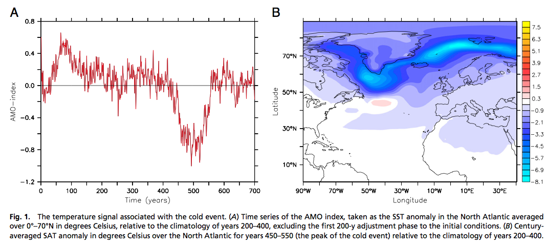
From Drijfhout et al 2013
Figure 1 – Click to expand
In their summary they state:
The lesson learned from this study is that the climate system is capable of generating large, abrupt climate excursions without externally imposed perturbations. Also, because such episodic events occur spontaneously, they may have limited predictability.
Before we look at the “causes” – the climate mechanisms – of this event, let’s briefly look at the climate model.
Their coupled GCM has an atmospheric resolution of just over 1º x 1º with 62 vertical levels, and the ocean has a resolution of 1º in the extra-tropics, increasing to 0.3º near the equator. The ocean has 42 vertical levels, with the top 200m of the ocean represented by 20 equally spaced 10m levels.
The GHGs and aerosols are set at pre-industrial 1860 values and don’t change over the 1,125 year simulation. There are no “flux adjustments” (no need for artificial momentum and energy additions to keep the model stable as with many older models).
See note 1 for a fuller description and the paper in the references for a full description.
The simulated event itself:
After 450 y, an abrupt cooling event occurred, with a clear signal in the Atlantic multidecadal oscillation (AMO). In the instrumental record, the amplitude of the AMO since the 1850s is about 0.4 °C, its SD 0.2 °C. During the event simulated here, the AMO index dropped by 0.8 °C for about a century..
How did this abrupt change take place?
The main mechanism was a change in the Atlantic Meridional Overturning Current (AMOC), also known as the Thermohaline circulation. The AMOC raises a nice example of the sensitivity of climate. The AMOC brings warmer water from the tropics into higher latitudes. A necessary driver of this process is the intensity of deep convection in high latitudes (sinking dense water) which in turn depends on two factors – temperature and salinity. More importantly, more accurately, it depends on the competing differences in anomalies of temperature and salinity
To shut down deep convection, the density of the surface water must decrease. In the temperature range of 7–12 °C, typical for the Labrador Sea, the SST anomaly in degrees Celsius has to be roughly 5 times the sea surface salinity (SSS) anomaly in practical salinity units for density compensation to occur. The SST anomaly was only about twice that of the SSS anomaly; the density anomaly was therefore mostly determined by the salinity anomaly.
In the figure below we see (left) the AMOC time series at two locations with the reduction during the cold century, and (right) the anomaly by depth and latitude for the “cold century” vs the climatology for years 200-400:
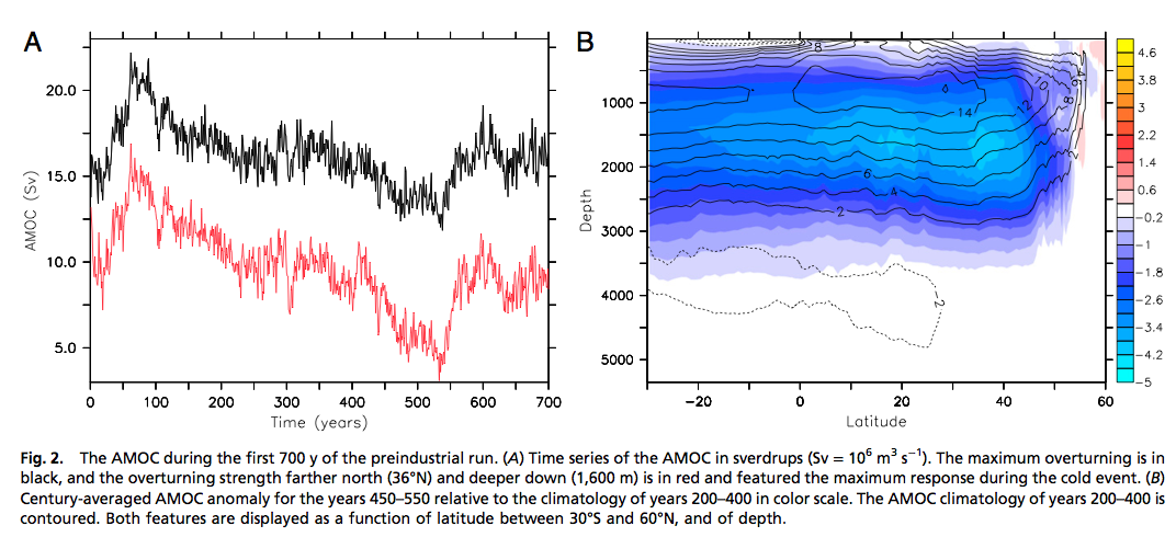
From Drijfhout et al 2013
Figure 2 – Click to expand
What caused the lower salinities? It was more sea ice, melting in the right location. The excess sea ice was caused by positive feedback between atmospheric and ocean conditions “locking in” a particular pattern. The paper has a detailed explanation with graphics of the pressure anomalies which is hard to reduce to anything more succinct, apart from their abstract:
Initial cooling started with a period of enhanced atmospheric blocking over the eastern subpolar gyre.
In response, a southward progression of the sea-ice margin occurred, and the sea-level pressure anomaly was locked to the sea-ice margin through thermal forcing. The cold-core high steered more cold air to the area, reinforcing the sea-ice concentration anomaly east of Greenland.
The sea-ice surplus was carried southward by ocean currents around the tip of Greenland. South of 70°N, sea ice already started melting and the associated freshwater anomaly was carried to the Labrador Sea, shutting off deep convection. There, surface waters were exposed longer to atmospheric cooling and sea surface temperature dropped, causing an even larger thermally forced high above the Labrador Sea.
Conclusion
It is fascinating to see a climate model reproducing an example of abrupt climate change. There are a few contexts to suggest for this result.
1. From the context of timescale we could ask how often these events take place, or what pre-conditions are necessary. The only way to gather meaningful statistics is for large ensemble runs of considerable length – perhaps thousands of “perturbed physics” runs each of 100,000 years length. This is far out of reach for processing power at the moment. I picked some arbitrary numbers – until the statistics start to converge and match what we see from paleoclimatology studies we don’t know if we have covered the “terrain”.
Or perhaps only five runs of 1,000 years are needed to completely solve the problem (I’m kidding).
2. From the context of resolution – as we achieve higher resolution in models we may find new phenomena emerging in climate models that did not appear before. For example, in ice age studies, coarser climate models could not achieve “perennial snow cover” at high latitudes (as a pre-condition for ice age inception), but higher resolution climate models have achieved this first step. (See Ghosts of Climates Past – Part Seven – GCM I & Part Eight – GCM II).
As a comparison on resolution, the 2,000 year El Nino study we saw in Part Six of this series had an atmospheric resolution of 2.5º x 2.0º with 24 levels.
However, we might also find that as the resolution progressively increases (with the inevitable march of processing power) phenomena that appear at one resolution disappear at yet higher resolutions. This is an opinion, but if you ask people who have experience with computational fluid dynamics I expect they will say this would not be surprising.
3. Other models might reach similar or higher resolution and never get this kind of result and demonstrate the flaw in the EC-Earth model that allowed this “Little Ice Age” result to occur. Or the reverse.
As the authors say:
As a result, only coupled climate models that are capable of realistically simulating atmospheric blocking in relation to sea-ice variations feature the enhanced sensitivity to internal fluctuations that may temporarily drive the climate system to a state that is far beyond its standard range of natural variability.
Articles in the Series
Natural Variability and Chaos – One – Introduction
Natural Variability and Chaos – Two – Lorenz 1963
Natural Variability and Chaos – Three – Attribution & Fingerprints
Natural Variability and Chaos – Four – The Thirty Year Myth
Natural Variability and Chaos – Five – Why Should Observations match Models?
Natural Variability and Chaos – Six – El Nino
Natural Variability and Chaos – Seven – Attribution & Fingerprints Or Shadows?
Natural Variability and Chaos – Eight – Abrupt Change
References
Spontaneous abrupt climate change due to an atmospheric blocking–sea-ice–ocean feedback in an unforced climate model simulation, Sybren Drijfhout, Emily Gleeson, Henk A. Dijkstra & Valerie Livina, PNAS (2013) – free paper
EC-Earth V2.2: description and validation of a new seamless earth system prediction model, W. Hazeleger et al, Climate dynamics (2012) – free paper
Notes
Note 1: From the Supporting Information from their paper:
Climate Model and Numerical Simulation. The climate model used in this study is version 2.2 of the EC-Earth earth system model [see references] whose atmospheric component is based on cycle 31r1 of the European Centre for Medium-range Weather Forecasts (ECMWF) Integrated Forecasting System.
The atmospheric component runs at T159 horizontal spectral resolution (roughly 1.125°) and has 62 vertical levels. In the vertical a terrain-following mixed σ/pressure coordinate is used.
The Nucleus for European Modeling of the Ocean (NEMO), version V2, running in a tripolar configuration with a horizontal resolution of nominally 1° and equatorial refinement to 0.3° (2) is used for the ocean component of EC-Earth.
Vertical mixing is achieved by a turbulent kinetic energy scheme. The vertical z coordinate features a partial step implementation, and a bottom boundary scheme mixes dense water down bottom slopes. Tracer advection is accomplished by a positive definite scheme, which does not produce spurious negative values.
The model does not resolve eddies, but eddy-induced tracer advection is parameterized (3). The ocean is divided into 42 vertical levels, spaced by ∼10 m in the upper 200 m, and thereafter increasing with depth. NEMO incorporates the Louvain-la-Neuve sea-ice model LIM2 (4), which uses the same grid as the ocean model. LIM2 treats sea ice as a 2D viscous-plastic continuum that transmits stresses between the ocean and atmosphere. Thermodynamically it consists of a snow and an ice layer.
Heat storage, heat conduction, snow–ice transformation, nonuniform snow and ice distributions, and albedo are accounted for by subgrid-scale parameterizations.
The ocean, ice, land, and atmosphere are coupled through the Ocean, Atmosphere, Sea Ice, Soil 3 coupler (5). No flux adjustments are applied to the model, resulting in a physical consistency between surface fluxes and meridional transports.
The present preindustrial (PI) run was conducted by Met Éireann and comprised 1,125 y. The ocean was initialized from the World Ocean Atlas 2001 climatology (6). The atmosphere used the 40-year ECMWF Re-Analysis of January 1, 1979, as the initial state with permanent PI (1850) greenhouse gas (280 ppm) and aerosol concentrations.


Interesting article, thank you.
Is it likely the GHG emissions we’ve released so far have reduced the probability of an abrupt cooling event.
For policy analysis I suggest we need pdfs for:
time (years) to the next abrupt change
Direction of the next abrupt change (to cooler or warmer)
rate of change
duration of change
total magnitude of change
which hemisphere
Figure 15.21 here http://eprints.maynoothuniversity.ie/1983/1/McCarron.pdf shows how often and how abruptly the climate changed between 16,000 and 11,000 years ago, and how much more stable it has been since it warmed up. More evidence warming is to be preferred over cooling?
Simple mechanisms – ice, cloud, dust, vegetation – combine to evolve in complex ways. The theory of abrupt climate change suggests that the system is pushed by changes in the system – past a threshold at which stage the components start to interact chaotically in multiple and changing negative and positive feedbacks – as tremendous energies cascade through powerful subsystems. Some of these changes have a regularity within broad limits and the planet responds with a broad regularity in changes of ice, cloud, Atlantic thermohaline circulation and ocean and atmospheric circulation. Abrupt change is defined as change that proceeds at a rate determined by the system itself and not external forcing.
There are theoretically indicators of approaching abrupt changes – e.g. http://www.pnas.org/content/105/38/14308.full . But little to suggest a methodology for predicting the onset and evolution of abrupt change.
For large scale changes – it is probably best to keep an eye on AMOC.
Click to access os-10-29-2014.pdf
Blocking patterns associated with the Arctic Oscillation seem to be involved. It is suggested that Arctic temperature amplification increases the frequency of blocking patterns – and increased spring melt reduces salinity in high latitudes. Conditions seem primed for a reduction in AMOC this century.
Following on from comment on the earlier thread I think the policy user will be less demanding than this.
What they want to know about is events with significant consequences that are out of the ordinary over the next 100 years. They need to be high risk (likelihood X consequence) to be of interest.
To give a couple of examples, gradual change is not a problem – see level rise continuing at current rates are risks that the population at large adapts to. On the other hand there might be a finite chance of another full blown ice age. Don’t bother us with that – equally a comet might break the earth in two.
On the other hand a gradual decline into another LIA may or may not be of concern.
Understanding what those events might be is therefore the starting point but, to repeat, within the constraint of today’s initial conditions and a time horizon of a hundred years. Characterised like this one wants to know what extreme boundaries are likely to be exceeded.
If we can’t predict the probability today then the policy makers is interested in how these conditions might evolve, so there is early warning. Doing nothing and watching in the face of uncertainty is a very useful strategy.
I suspect considering the analogy with the management and study of seismic risks is useful. Living in a country exposed to these we have a well developed sense of how a community deals with large, uncertainty but foreseeable risks. We accept and manage with the small stuff, we don’t worry about the predicable stuff (eg slow earthquakes), and we put effort into understanding impact and likelihood of the big ones (earthquakes, Tsunamis) and into managing the consequences, and if Lake Taupo blows again – so long and thanks for the fish.
Bringing this back to the subject of these various threads it might be interesting to look at the extent to which chaos theory has contributed to the understanding of events and their precursors in that domain.
Intended as a reply to Peter Lang January 4, 2015 at 8:59 am
HAS,
Thank you. Interesting points and an excellent analogy with the handling of earthquake risks. I’ll use that one.
I haven;t read the previous posts on Science of Doom. I was pointed here by a link on Climate Etc.
My perspective is largely driven policy analysis, especially about what sort of policies are achievable and politically sustainable. There is a strong push by those most concerned about CAGW to have UN imposed regulations (with penalties for breach of commitments) or pricing of GHG emissions. I believe there is negligible chance of such policies succeeding in achieving the stated objectives – i.e. reduced climate damages. Only policies that are economically beneficial irrespective of any assumed climate damages avoided can succeed.
I was also lead to this articles yesterday. The chart at slide #9 on the presentation is interesting (IMO):
http://canadianenergyissues.com/2014/01/29/how-much-does-it-cost-to-reduce-carbon-emissions-a-primer-on-electricity-infrastructure-planning-in-the-age-of-climate-change/
Peter,
My fundamental principle of human events is that irony always increases. Slide #13 in your linked article is yet more proof that this is true.
DeWitt Payne,
I’m a huge fan of irony, so thanks for the highlight.
http://www.nap.edu/openbook.php?record_id=10136&page=1
Solutions involve reducing anthropogenic changes on the system and are multi-dimensional involving economic and social development, better land use practices, sustainable production systems, reduction of population pressures, technological innovation and ecological restoration.
http://thebreakthrough.org/archive/climate_pragmatism_innovation
Creative responses that build on social and economic development and enhance resilience – while reducing pressures on the system – would seem the rational way to go.
The Copenhagen Consensus post 2015 MDG goals – focusing on the most effective use of existing commitments – would seem to be a good place to start.
http://www.copenhagenconsensus.com/post-2015-consensus
Are these ‘climate excursions’ one-sided? Are the extreme climate fluctuations only on the cooling side? Any evidence of rapid heating (similar in magnitude to the second half of the 20th C) in pre-history?
Nathan,
This one is a cooling – but as the article says, climate models generally don’t produce these abrupt changes.
Of course, when they do, it might be assumed that there is a problem, rather than a fabulous step forward (like penicillin).
For example in Natural Variability and Chaos – Seven – Attribution & Fingerprints Or Shadows? where the simulation (red circled) in figure 1 was removed for being unphysical.
Don’t get me wrong, sometimes models produce spurious results and they are clearly spurious – an example of that is in the discussion on Models, On – and Off – the Catwalk – Part Four – Tuning & the Magic Behind the Scenes where we had a brief look at Uncertainty in predictions of the climate response to rising levels of greenhouse gases, Stainforth et al, Nature (2005).
But like with removing trends because models often drift, if we remove abrupt changes because models have convergence and paramaterization issues we might find, on reflection, that we have thrown the baby out with the bathwater.
The lead author of the paper, Sybren Drijfhout, has kindly offered to dig out a few recent papers which show some kind of abrupt change (in models).
I am enjoying the explorations you do, so thanks.
My questions is not really about whether the models can reproduce these events (if they’re rare, shouldn’t they also be rare in models?).
What I am asking is there evidence in paleoclimate of a warming event of equivalent magnitude to the DO events. So was just wondering if it was possible that the ‘natural variation’ is mostly on the cooling side. Or if events of this magnitude are generally cold, rather than hot.
Is there a reason they should (would/must) be equal in both directions?
Wasn’t this study was done with a preindustrial CO2 level? In earlier discussions on examples of abrupt climate change, I don’t see that the LIA is mentioned as an example. The definition of abrupt climate change has been changing. Where will this sliding definition end? Will early 20th century warming (1910 to 1940) be an example of abrupt climate change? Whatever happens in the 21st century will happen with CO2 at 395 ppm, or higher. If CO2 drops 20 to 40 ppm because of an AMOC shutdown, how far will the GMT drop? I have read papers that indicate it’s unlikely there will be a shutdown of the AMOC in the 21st century, and, if there should be one, the drop in GMT will be modest. Maybe that all wrong and the right answer was tossed out. Maybe.
Nathan,
Not that I know of. I haven’t investigated any skewness and I haven’t seen any discussion of skewness in any papers, but I don’t have evidence either way.
JCH
Yes, that’s typical for doing “control runs” of “internal variability” in climate models.
?? Are you talking about papers on paleoclimate?? Can you cite some examples?
If you are talking about websites and blogs, no need, it’s irrelevant to this site.
I don’t understand the rest of your comment.
As a brief, possibly irrelevant perspective:
A lot of studies have focused on the shutdown of the AMOC as a mechanism for abrupt change. GCMs have mostly struggled to shutdown the AMOC even with large changes in CO2 (quadrupling CO2). GCMs experiments have tried “big time hosing” of freshwater into the high northern latitudes and have succeeded in large changes in the AMOC, causing significant temperature change. The AMOC later recovers in these freshwater hosing experiments.
This particular experiment is quite different.
The climate is meandering along, minding its own business when suddenly something “abrupt” happens. It’s quite different from the experiments with instantaneous 4xCO2 and from the experiments with big time freshwater pouring into the high latitude oceans.
Is Science Of Doom a blog? Is this a circular irrelevancy?
Is WHT actually a creature thought to be mythical and said to live under bridges?
I learn a great deal from reading papers I find on google scholar. For instance, papers by Broecker, a few of which I read a couple of years ago when RC posted an article about Broecker. In those papers Broecker makes no mention of the LIA being an example of abrupt climate change.
last night I did find a magazine article where Broecker does discuss the LIA in the context discussed here.
As scientists, our first responsibility is to examine facts, and then draw preliminary conclusions. We then develop a hypothesis to try to explain why the facts observed occur. If at some point more supporting facts develop, and no contradiction to our hypothesis occurs, we may call the hypothesis a theory.
If no reliable supporting real evidence is obtained, and in fact contradictions to the hypothesis occur, a change in hypothesis is clearly needed. The CAGW hypothesis, and in fact the AGW hypothesis seemed initially supported by the fact of increasing CO2 (which is reasonably connected to human activity), and the fact that CO2 is an absorbing gas, and due to the rising overall trend of temperature in the last century (all facts so far). Initial looks at longer trends seemed to indicate those trends as very unusual. Computer models seemed to support the hypothesis that increasing CO2 and likely positive feedback from increased water vapor would lead to a major problem if something was not done to slow or stop it from rising more.
Later work now supports that the warming trend (which stopped around the beginning of the 21st century) does not seem unusual over the last 10,000 or so years, and certainly not on longer time scales, even as to rate of change. Many indicators such as melting sea ice reversed, and in fact evidence of frequent prior melting makes the recent melting not unusual. Actual measurements of water vapor do show increase associated with the temperature increase, but mainly at low altitudes, where they have little effect on added temperature, and in fact variation in clouds may totally dominate the CO2 and water vapor effects. Computer models (developed at a total cost of many billion dollars) have shown no skill at global or regional scales.
Based on the above, reasonable scientists would conclude the CAGW or even the AGW hypothesis is badly flawed. Instead, many scientists, politicians, and others, cling to a falsified position, bringing up many flawed statements, and some even attack verbally the skeptics (who are supported by facts). Rob Ellison ended with “The Copenhagen Consensus post 2015 MDG goals – focusing on the most effective use of existing commitments – would seem to be a good place to start.” This is a typical holding on to a flawed position, rather than being more realistic and adopting the physicians motto: “first do no harm”, which means in this case: wait and see rather than doing anything.
It is probably just as likely that it will cool, not heat in the future (we are likely close to the end of the Holocene, based on previous interglacial periods), and cold is far worse that warm. Also the added CO2 has had enormous beneficial value on crops, and lowering it from the present level would contribute to loss of productivity. If the many billions of dollars wasted on studies, meetings, and physical efforts to cut CO2 production in the last several decades had been spent on real pollution control, and positive humanitarian work, it would have done much more good. Limiting growth in third world countries in order to hold down CO2 is one of the most self destructive actions made in recent times.
ummmm… Probably not the place to have this sort of rant.
‘The crash of 2009 presents an immense opportunity to set climate policy free to fly at last. The principal motivation and purpose of this Paper is to explain and to advance this opportunity. To do so involves understanding and accepting a startling proposition. It is now plain that it is not possible to have a ‘climate policy’ that has emissions reductions as the all encompassing goal.
However, there are many other reasons why the decarbonisation of the global economy is highly desirable. Therefore, the Paper advocates a radical reframing – an inverting – of approach: accepting that decarbonisation will only be achieved successfully as a benefit contingent upon other goals which are politically attractive and relentlessly pragmatic.
The Paper therefore proposes that the organising principle of our effort should be the raising up of human dignity via three overarching objectives: ensuring energy access for all; ensuring that we develop in a manner that does not undermine the essential functioning of the Earth system; ensuring that our societies are adequately equipped to withstand the risks and dangers that come from all the vagaries of climate, whatever their cause may be.
It explains radical and practical ways to reduce non-CO2 human forcing of climate. It argues that improved climate risk management is a valid policy goal, and is not simply congruent with carbon policy. It explains the political prerequisite of energy efficiency strategies as a first step and documents how this can achieve real emissions reductions. But, above all, it emphasises the primacy of accelerating decarbonisation of energy supply.
This calls for very substantially increased investment in innovation in non-carbon energy sources in order to diversify energy supply technologies. The ultimate goal of doing this is to develop non-carbon energy supplies at unsubsidised costs less than those using fossil fuels.
Click to access HartwellPaper_English_version.pdf
There is $2.5 trillion slated for aid to 2030. Progress can be made while focusing on humanitarian and environmental objectives.
The purpose of the rant is based on the fact that despite no real evidence of CAGW or significant AGW, the default position continues to be assume it is likely to warm, although not clear how fast or much, and do things that tend to minimize warming. If it cools instead, any movement to prepare for warming would make things worse, and lack of preparing for the possibility of cooling would be a problem. I am trying to get responses that admit we should look at all eventualities. Huge amounts of money are being spent on the warming “problem”, and studies are mostly one sided. This lack of scientific honesty should not be ignored. I greatly respect SOD and many of the responders, as trying to get to the truth, but most still assume the warming problem, and concentrate on what governments should do.
Leonard,
Looking at previous interglacial periods in the Vostok ice core, if it were going to cool, it would have started thousands of years ago. But things like atmospheric methane have broken out of the decay pattern previously observed. That’s why Ruddiman hypothesized that the land use changes and methane emission from rice paddies from the invention of agriculture 8,000 years ago has already altered the climate.
DeWitt,
The Holocene started over 10,000 years ago. The unusual relative top hat pattern of the Holocene temperature (compared to several previous interglacial periods) was evident from the beginning of this cycle. In fact, going back several cycles, there were periods as long or longer than present (depending where you pick the thresholds). Methane has collected and been released in large scale before and did not cause temperature spikes (except possibly the PETM, but this was at elevated temperatures already). Ruddiman makes an interesting hypothesis but has no realistic supporting evidence. The Methane level during the Holocene is available from the ice records, and is not that unusual. Since Methane decomposes rapidly in sunlight to CO2, the CO2 should also have spiked. This is also a record in the ice, and is claimed to be below 200 ppm this whole time, and not changed except recently. I do agree the human activity may delay or soften onset of cooling somewhat, but that is a good thing.
There are natural causes for glacials of course. Warming at high latitudes increase ice clear areas, increased evaporation, higher winter snowfall, higher spring melts and lower salinities in the Arctic and declining AMOC. Are we adding to that? The models certainly suggest so.
In conditions of low NH insolation and low AMOC – snow survives the summer melt and ice sheets spread rapidly. Multiple feedbacks from multiple conceptually simple mechanisms resulting in abrupt and more or less extreme global and regional change that is quite unpredictable.
On the other hand reducing energy costs through research, reducing black carbon, restoring carbon levels in agricultural soils and restoring ecosystems has nothing but predictable economic growth, health, agricultural productivity and environmental outcomes.
By stopping emissions we might make things worse? If a cheap and abundant low carbon energy source power were discovered tomorrow – you would reject it? Thus we see the descent into absurdity.
By rational multi-objective policy we might make things a hell of a lot better,
http://www.nap.edu/openbook.php?record_id=10136&page=1
http://thebreakthrough.org/archive/climate_pragmatism_innovation
Rob,
It is more likely that human caused mild warming would reduce, not increase rapid changes in most strong weather. Remember that most warming (whatever cause) occurs at higher latitudes, at night, and in winter. These do not mostly happen during day, summer, and lower latitudes. This decrease in gradients decreases driving forces for storms, and other weather related sudden events. If the change were large enough, it would likely cause a shift in the latitude where rain and dry weather occur over time, so disruption of some types would occur, but probably slow enough that modern society could adapt. So called no regret policies do have potential for large regret.
Missed the place – https://scienceofdoom.com/2015/01/04/natural-variability-and-chaos-eight-abrupt-change/#comment-90344
What does GHG warming do to the temperature gradient between the surface and the stratosphere? What consequences might that change have for storm intensity?
Leonard: While there are many problems GCMs and with CAGW, do you have any reason to believe that the radiative imbalance due to accumulating GHGs will not produce an warmer climate when the current episode of natural variability has come to an end?
Frank
How do you define a warmer global climate?
This is a serious question. As I’ve asked before how many different climates have we had over the last couple of thousand years, what defined them and when did we have them?
And come to that what do you think the next climate we will get will be and how will we recognise it as being different from our current climate (and how are we defining that)?
HAS asked me to define “warmer”. Let’s take the average of temperature of the hiatus period (or 2001-2010) and add 0.2 degC (a decade’s worth of warming for the IPCC’s models). That would be warmer to me.
My emphasis was more on the word “climate”.
You see 0.2 C warmer is surely within the realm of weather. At what point do we move to a different climate?
Frank: While CO2 accumulation alone would cause a slight increase in the temperature that would otherwise occur, the feedbacks may reduce or increase the effect (we do not know which way feedbacks go, but large positive feedback is very unlikely or climate would not be as stable over time as it has). However, notice the statement “that would otherwise occur”. The trend of natural variation may be down enough so that the small CO2 additional effect would only slightly slow the down trend, not make it go up. The point is that unknown feedbacks on a small effect, and possibly large natural trends dominate, so we do not know which way temperature will go.
Leonard,
High natural variability and low climate sensitivity are probably mutually exclusive, especially if you invoke large (unknown) negative feedbacks to explain low sensitivity. Otherwise, you have to posit a feedback that is only effective for ghg radiative forcing and no other form of temperature change. Would you care to explain how that would work?
The second the high trade winds (England) that have dominated the 2000s stop blowing, the surface air temperature starts going up at multiples of the IPCC’s.2C per decade. They calmed near the end of 2012, and warming rate since then is:
slope = 0.0628235 per year
And that’s how you get a warmest year in the instrument record with no El Nino.
What in natural thing caused the surface to warm at a rate of .63C per decade since 2012?
DeWitt (Jan 10, 3:12 pm). You have got to be kidding. The variation the last 600 MY, the variation the last 3 MY (period of ice records), and even the last 10 KY (Holocene) have huge variations, most of which are not understood. We can talk about about land mass drift, Earth tilt, and other factors, but even over shorter periods where these are not obvious, large variation occurs for which we have no forcing to explain. During glacial periods between the interglacial periods, huge up and down variations occur. The Earth, ocean, and ice energy storage and release, large scale ocean current variations over long and short times, cloud variations, and just the nature of response of non-linear multidimensional systems cause large variations of many time scales. This is the nature of such chaotic systems. When you include the possible solar variation (UV or cosmic ray effects, not average intensity), and the effect of biological processes, the problem is even more complex.
You keep invoking the need for forcing and feedback. We do not know even if these are significant compared to natural (i.e., non human caused but not understood) variations. If the small forcing and feedback are of slight short term effect, it is likely that cloud variation negative feedback reduces water vapor increase positive feedback, and CO2 alone is a small effect to start with. When you include aerosols, the CO2 and feedback total may be very small, and easily dominated by natural variation.
At the present there is no supporting evidence that human activity has even a clear measurable net effect. If you can show otherwise, please do so.
Leonard,
Your reply is nonsense. I won’t bother trying to explain why as you’re clearly incapable of understanding.
Leonard: Unfortunately, anthropogenic increases in GHGs are likely to produce a future forcing change of about 4 W/m2 by the end of the century. There is good evidence from space for at least some positive feedback in OLR from clear skies (water vapor plus lapse rate) and no evidence for strongly-negative cloud feedback. This seems to be consist with lower estimates of climate sensitivity from energy balance models. However, even with a TCR of 1.35 degC and ECS of 1.8-2.0, GHG-driven warming with be about 2/3 as much as the IPCC’s central estimates. So I find it difficult to reconcile these numbers with your more optimistic, but less quantitative, views. There appears to be some prospect of lower solar activity in the near future, but even another Maunder Minimum appears incapable of preventing future warming.
Nathan,
“What I am asking is there evidence in paleoclimate of a warming event of equivalent magnitude to the DO events. So was just wondering if it was possible that the ‘natural variation’ is mostly on the cooling side. Or if events of this magnitude are generally cold, rather than hot.”
Surely the best-studied sudden warming event in recent geological history is the end of the Younger Dryas. I’m not certain about recent developments in this area, but there was a letter to Nature about 20 years ago that talked about ice core evidence for warming in Greenland of some 7 C over a period of 20 years or less. They also hint that the transition from the Oldest Dryas to the warm period that followed was similarly abrupt. I’ve only read the abstract, unfortunately, since the paper itself is paywalled.
http://www.nature.com/nature/journal/v362/n6420/abs/362527a0.html
Elisat
Freaky! That’s a sudden warming… Wonder what that amounted to as a ‘global’ change.
It’s not clear whether the YD was even a global cooling event, though there is evidence of climate change at many sites worldwide. RealClimate has talked about the period a few times; the most recent one that I know of is linked below.
http://www.realclimate.org/index.php/archives/2010/07/revisiting-the-younger-dryas/
Science of Doom,
None of my comments were meant to belittle your excellent work. You do a good job of realistically examining each piece in the issue. My comments here were an effort to engage discussion since your responders are smart people.
Science of Doom
Can you comment on the latest paper of Miscolczi. Judith Curry mentioned it in her blog and asked for comments. Thanks.
Dr. Strangelove,
I looked in detail at previous papers.
They weren’t very good. An awful and flawed understanding of theory and a poor application of experimental results.
Does the new paper start off by addressing the problems of his earlier papers?
Let me know why you think this one is an improvement.
SOD: You might be interested to note that Miscolczi referenced discussions at your blog (and DeWItt and Eli by name) in his latest paper.
It seems that he has extended is previous work to include cloudy skies. I noted that his clouds are infinitely thin and radiate the same amount of energy both up and down.
Frank,
Except clouds are not thin and don’t radiate equally upward and downward. Cloud tops are cooler than cloud bottoms so there is less radiation upward than downward. Then there’s absorption, reflection and scattering of incoming solar radiation, all of which depend on clouds having significant thickness, with thickness having the most effect on scattering. In the near UV and visible, absorption is insignificant, so scattering determines the fraction of light that is transmitted, forward scattered, and reflected.
IMO, the major problem of most, if not all, climate models is that cloud feedback is positive. In other words, if the Earth were completely cloud covered, the surface temperature would be higher than it is now. Clouds radiate less than the surface with clear sky, but not that much less. Cloud positive feedback is probably also why the modeled ECS is so much larger than the TCR and isn’t linear with forcing. In fact, after looking at some of Kenneth Fritsch’s work at The Blackboard (see for example this comment as well as others in this thread), I find model ECS to be a complete joke, worse than a guess.
MODTRAN is something of a blunt instrument, but for the tropical atmosphere, clear sky, all other settings default, upward radiation at 70km is 289.288 W/m². With the first cumulus cloud setting, it drops to 262.002 W/m². That’s a drop of less than 10%. And even in a totally cloud covered world, surface reflectivity would still be important for the incoming transmitted radiation.
DeWitt: Thanks for the link to Kenneth’s work. As I am sure you know, most climate models don’t conserve energy; they show a radiative imbalance even though surface temperature has stabilized early in the control run. After quadrupling CO2, how do they know the built-in energy loss or gain will remain the same?
I shouldn’t be cynical, but someday we may find that climate models are as problematic as the paleoclimatologists reconstructing temperature from proxy data. Both groups are driven by political pressures: The latter wanted to prove that the current warm period is warmer than the MWP. The former need to provide policymakers useful answers about how climate will change when CO2 doubles and triples. They have been lavishly funded for decades, but I doubt their output would be considered acceptable for policy making if they were candid about all of the problems they haven’t solved. Until AR3 or AR4, they needed flux adjustment. AR4 wasn’t candid about the uncertainty associate with parameters. Apparently all AR5 models are too sensitive to aerosols. The use of temperature anomalies disguises the fact that they disagree about GMST.
Figures 3 and 4 of the Manabe PNAS paper linked below show just how poorly and inconsistently CMIP3 and CMIP5 models reproduce the annual cycle of changes in TOA fluxes (LWR and reflected SWR) during the ERBE and CERES era. Most models slightly exaggerate clear sky LWR feedback (water vapor plus lapse rate) and get everything else seriously wrong in different ways.
http://www.pnas.org/content/110/19/7568.full
Frank
“…climate models are as problematic as the paleoclimatologists reconstructing temperature from proxy data …. wanted to prove that the current warm period is warmer than the MWP”
There are exceptions:
A team of paleoceanographers, lead by Dalia Oppo of Woods Hole Oceanographic Institute, concluded in 2009 that the MWP was indeed warmer than current temperatures.
http://www.whoi.edu/main/news-releases/2009?tid=3622&cid=59106
Richard
RichardS: One should always be cautious the often-exaggerated claims appearing in the blogosphere (and even the politicized portions of the “scientific press”) about the importance of any one paper. The full text of a Oppo (2013) can be found here:
Click to access yair_2013.pdf
The sediment cores they use come from the ocean near Indonesia, but are supposed to be representative of a larger portion of the planet. Like other “teleconnections”, the reasoning is pretty convoluted and there is no way to prove that the foraminifer that grew there in the past were responding in the same way to a near-global temperature signal:
“We use a suite of sediment cores along bathymetric transects in the Makassar Strait and Flores Sea in Indonesia (figs. S1 and S2) to document changes in the temperature of western equatorial Pacific subsurface and intermediate water masses throughout the Holocene [0 to 10 thousand years before the present (ky B.P.)] (Table 1). This region is well suited to reconstruct Pacific OHC, as thermocline and intermediate water masses found here form in the mid- and high-latitudes of both the northern and southern Pacific Ocean and can be traced by their distinctive salinity and density as they flow toward the equator (7) (fig. S3). The Makassar Strait between Borneo and Sulawesi, the Lifamatola Passage east of Sulawesi on the northern side of the Indonesian archipelago, and the Ombai and Timor Passages to the south serve as major conduits for exchange of water between the Pacific and Indian Oceans; water flow through these passages is collectively referred to as the Indonesian Throughflow (ITF) (8). The upper thermocline component of the ITF (~0 to 200 m) is dominated by contributions from North Pacific and, to a lesser extent, South Pacific subtropical waters, marked by a subsurface salinity maximum (figs. S3 and S4). Within the lower thermocline (~200 to 500 m) the inflow of low-salinity North Pacific Intermediate Water (NPIW) dominates the ITF flow (fig. S4). The higher- and relatively uniform–salinity water below the main thermo- cline (~450 to 1000 m) is referred to as Indo- nesian Intermediate Water, which is formed in the Banda Sea by strong vertical mixing between shal- low, warm, relatively fresh waters and deep, cold, relatively salty waters (8, 9). At intermediate depths, the Banda Sea gets contributions from the South Pacific through the northwestward-flowing New Guinea Coastal Undercurrent (NGCUC). Studies suggest that the NGCUC carries a substantial contribution from the Antarctic Intermediate Water, spreading into the Banda Sea through the Lifamatola and Makassar passages (10). The main subthermocline outflows through the Timor and Ombai passages reverse intermittently, thereby allowing inflow of Indian Ocean water into the Indonesian seas (8, 11, 12). Thus, the hydrography of intermediate water in this region is linked to and influenced by surface conditions in the high latitudes of the Pacific Ocean, as is also sug- gested from the distribution of anthropogenically produced chlorofluorocarbon along these isopycnal layers (7).”
Fortunately, it doesn’t make much difference whether the MWP was or was not warmer than today or whether paleoclimatologists have accurately conveyed the uncertainties associated with their work. Future climate change depends on natural variability (which we can’t control), anthropogenic forcing agents (which we can control) and climate sensitivity. So mischaracterization of the reliability of and uncertainty in the output from climate models is a far bigger problem than the MWP.
Frank
Thank you for the link.
I do not think the study is saying that the sediment cores are representative of the planet. Here, I believe, is a relevant passage:
“The reconstructed OHC is compared with modern observations for the whole Pacific at the same depth range (5). The comparison suggests that Pacific OHC was substantially higher during most of the Holocene than in the past decade (2000 to 2010), with the exception of the LIA. The difference is statistically significant, even if the OHC changes apply only to the western Pacific…”
Also, from my understanding, there is a strong relationship between proxy reconstructions and model outputs. The models start with “an estimate of internal variability” which appears to rely on paleoceanography data.
Regards,
Richard
RichardS: You said that a team of paleoceanographers concluded that the MWP was indeed warmer than current temperatures. Fortunately, you didn’t specify whether you meant globally, regionally or locally warmer. However, it is possible to get a misleading ideas from:
Or, you could get a more balanced view from Judith Curry, but her post states that it was written without access to the paper itself.
Or, you can learn that this paper demonstrates that the current rate of ocean warming is unprecedented in the last 10,000 years.
http://www.skepticalscience.com/oceans-heating-up-faster-than-past-10000-years.html
In this politicized environment, it usually makes sense to attempt to verify extraordinary claims with the primary source.
Frank
You provided some interesting reading, thank you. You’re right. Not all reconstructions look the same and bias complicates the science. I may be wrong, but following Steve’s references and links, it appears that AR5 attribution relies on an “estimate of internal variability” that, in turn, relies on a paleoceanography reconstruction that is amazingly flat over the last 2k years.
I’m not smart enough to sort this out on my own, but perhaps an honest broker will set me straight.
Richard
Science of Doom
I just read the abstract and I already found a misunderstanding of the atmospheric greenhouse effect in the quotation below.
“In steady state, the planetary surface (as seen from space) shows no greenhouse effect: the all-sky surface up-ward radiation is equal to the available solar radiation.”
At equilibrium, the outgoing radiation is equal to the incoming solar radiation. It doesn’t mean there is no greenhouse effect. The temperature could have already increased to attain the equilibrium. Venus may be at radiative equilibrium since it’s not getting any hotter but it’s hot enough to melt lead due to greenhouse effect.
Also, the satellite measurements of TOA radiation are not accurate enough to detect small radiative imbalance. They can measure accurately changes in radiation flux not the absolute flux. Do say if you see more problems with the paper.
BTW another mistake in the quotation is the planetary surface. The radiative balance should be taken at TOA not at the surface since greenhouse effect is an atmospheric phenomenon.
I read the paper. His conclusion of no greenhouse effect is based on his computation of transmittance, which he called optical thickness and claims to be invariant. It is wrong because transmittance is not a measure of greenhouse effect. It is simply a ratio of energy coming in and going out of the atmosphere. It doesn’t tell us how much energy is in the atmosphere at any given time, which is the relevant quantity to determine temperature changes.
Sorry he derived the optical thickness from transmittance but two different quantities. Just the same. An invariant optical thickness, assuming it is true, does not disprove greenhouse effect.
Ratio of energy flow is irrelevant, absolute energy flow is. Example:
energy out / energy in
1/10
10/100
The two ratios above are equal but the 2nd fraction will have more energy in the system.
There are two fundamental errors in that argument of Miskolczi:
1) Optical thickness of the whole atmosphere does not determine the strength of GHE, the optical thickness of the upper troposphere is more essential, and that’s certainly affected by CO2 also in his calculations. (He may have skipped extracting that information, but I think that he knows the fact very well, just declines telling that.)
2) His argument that the optical thickness is constant is totally false. He mixes some observations with some theory based formulas in a totally obscure an inconsistent way. Distorting numbers and interpreting evidence for some upper limits for the change as evidence for exactly no change is an approach that can produce whatever result the author wishes.
I’m not going to bother reading the paper, but back when this was being discussed I found a fundamental error in the derivation of his theory. He treats an integration constant as a variable when he takes a derivative. All his conclusions follow from that mistake. But he’s probably so emotionally invested that he literally can’t see the problem.
While I don’t agree with all of his analysis, he does not claim there is no greenhouse effect. In fact, he basically claims that the water vapor for a mainly water covered planet self compensated to maintain a constant average greenhouse effect.
But that’s total nonsense. Without more warming of the surface there isn’t any more water vapor that would compensate at all the effect of additional CO2. Furthermore, even if the total optical depth of the atmosphere were unchanged the GHE would still get stronger, because the compensation would take place in the way that the lower troposphere would be more transparent while the changes of the upper troposphere are dominated by CO2. Thus is ideas are doubly nonsense.
Pekka: Miskolczi relies upon radiosonde data showing that the upper troposphere has become drier over the past few decades. The same data went to the NCEP re-analysis that Paltridge analyzed to reach the same conclusion. This conclusion is not “nonsense”, but the data on which it is based may be wrong. On his blog, Roy Spencer has stated that he has no confidence in the early radiosonde data that shows higher humidity in the upper troposphere.
Paltridge, G. W, A. Arking and M. Pook, Trends in middle- and upper-level tropospheric humidity from NCEP reanalysis data, Theor. Appl. Climatol., 98, 351-359, 2009.
Water vapor in the upper troposphere is not in equilibrium with liquid water and SSTs (or even the boundary layer) many kilometers below.
Also any claim of a constant GHE is almost certainly inconsistent with paleoclimate.
[…] « Natural Variability and Chaos – Eight – Abrupt Change […]
I liked the article very much. Perhaps I am wrong, but I think the number of Nazi victums was about 11 million,was it not – the 6 million being the Jews, who refer to their part as “the” holocost. The others counted to their relatives, one might expect, and are no less to be regretted..
Very interesting article. This is coming from an undergraduate student in mathematics who has an interest in pursuing fluid dynamics at some point. I’m curious — in the climate models being simulated, I am assuming they are computationally intensive (hence, your mentioning in this post that only a few hundred years have been computed etc.), but I’ve attended many lectures by astronomers and astrophysicists modeling supernovae “explosions.” Perhaps you might team up and see if you might learn something from one another? The equations are very similar, in fact in the astrophysicist’s case, even more difficult (there is a large magnetic field component and much higher temperatures and pressures involved in stars) it seems.