In (still) writing what was to be Part Six (Attribution in AR5 from the IPCC), I was working through Knutson et al 2013, one of the papers referenced by AR5. That paper in turn referenced Are historical records sufficient to constrain ENSO simulations? [link corrected] by Andrew Wittenberg (2009). This is a very interesting paper and I was glad to find it because it illustrates some of the points we have been looking at.
It’s an easy paper to read (and free) and so I recommend reading the whole paper.
The paper uses NOAA’s Geophysical Fluid Dynamics Laboratory (GFDL) CM2.1 global coupled atmosphere/ocean/land/ice GCM (see note 1 for reference and description):
CM2.1 played a prominent role in the third Coupled Model Intercomparison Project (CMIP3) and the Fourth Assessment of the Intergovernmental Panel on Climate Change (IPCC), and its tropical and ENSO simulations have consistently ranked among the world’s top GCMs [van Oldenborgh et al., 2005; Wittenberg et al., 2006; Guilyardi, 2006; Reichler and Kim, 2008].
The coupled pre-industrial control run is initialized as by Delworth et al. [2006], and then integrated for 2220 yr with fixed 1860 estimates of solar irradiance, land cover, and atmospheric composition; we focus here on just the last 2000 yr. This simulation required one full year to run on 60 processors at GFDL.
First of all we see the challenge for climate models – a reasonable resolution coupled GCM running just one 2000-year simulation consumed one year of multiple processor time.
Wittenberg shows the results in the graph below. At the top is our observational record going back 140 years, then below are the simulation results of the SST variation in the El Nino region broken into 20 century-long segments.
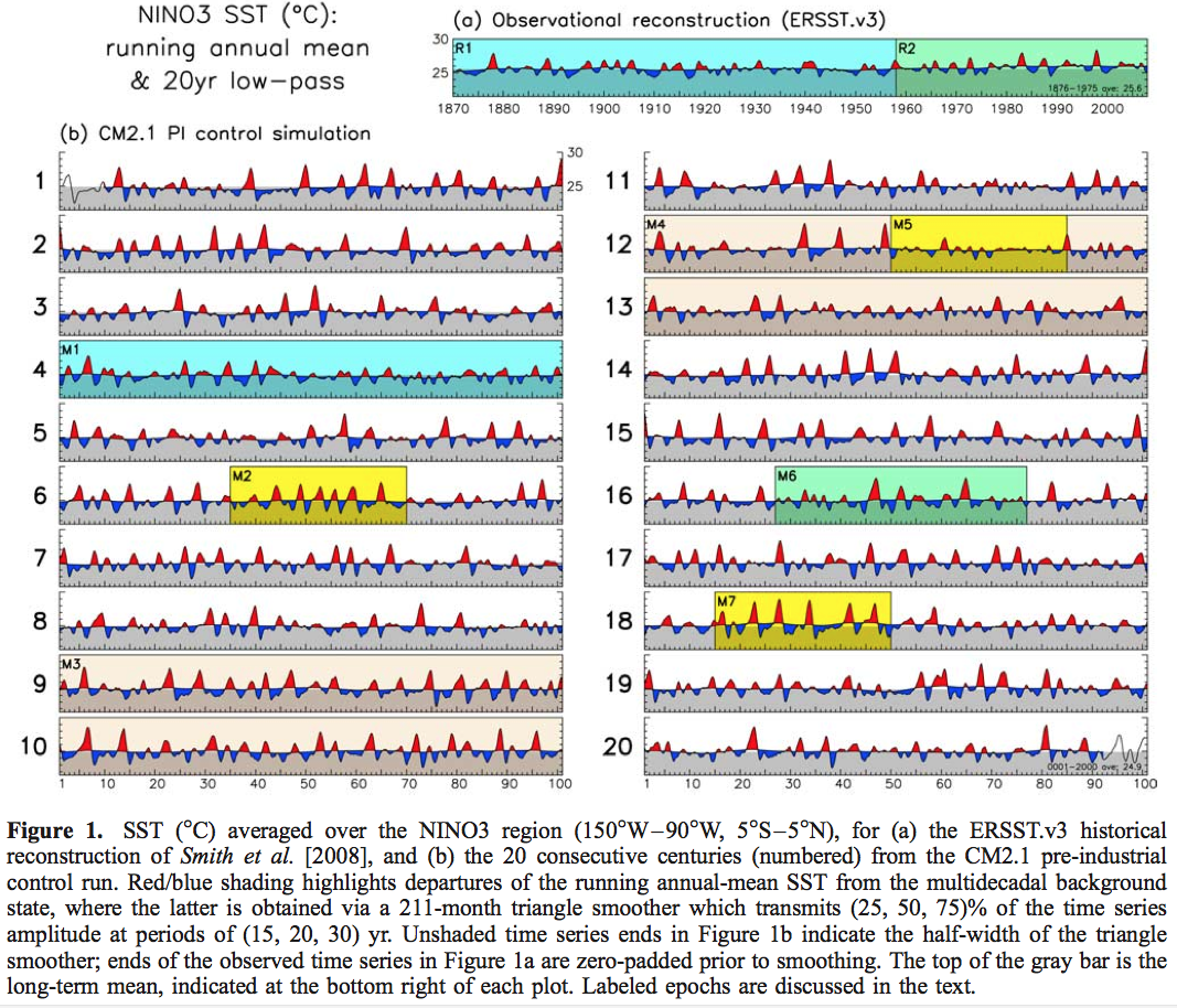
From Wittenberg 2009
Figure 1 – Click to Expand
What we see is that different centuries have very different results:
There are multidecadal epochs with hardly any variability (M5); epochs with intense, warm-skewed ENSO events spaced five or more years apart (M7); epochs with moderate, nearly sinusoidal ENSO events spaced three years apart (M2); and epochs that are highly irregular in amplitude and period (M6). Occasional epochs even mimic detailed temporal sequences of observed ENSO events; e.g., in both R2 and M6, there are decades of weak, biennial oscillations, followed by a large warm event, then several smaller events, another large warm event, and then a long quiet period. Although the model’s NINO3 SST variations are generally stronger than observed, there are long epochs (like M1) where the ENSO amplitude agrees well with observations (R1).
Wittenberg comments on the problem for climate modelers:
An unlucky modeler – who by chance had witnessed only M1-like variability throughout the first century of simulation – might have erroneously inferred that the model’s ENSO amplitude matched observations, when a longer simulation would have revealed a much stronger ENSO.
If the real-world ENSO is similarly modulated, then there is a more disturbing possibility. Had the research community been unlucky enough to observe an unrepresentative ENSO over the past 150 yr of measurements, then it might collectively have misjudged ENSO’s longer-term natural behavior. In that case, historically-observed statistics could be a poor guide for modelers, and observed trends in ENSO statistics might simply reflect natural variations..
..A 200 yr epoch of consistently strong variability (M3) can be followed, just one century later, by a 200 yr epoch of weak variability (M4). Documenting such extremes might thus require a 500+ yr record. Yet few modeling centers currently attempt simulations of that length when evaluating CGCMs under development – due to competing demands for high resolution, process completeness, and quick turnaround to permit exploration of model sensitivities.
Model developers thus might not even realize that a simulation manifested long-term ENSO modulation, until long after freezing the model development. Clearly this could hinder progress. An unlucky modeler – unaware of centennial ENSO modulation and misled by comparisons between short, unrepresentative model runs – might erroneously accept a degraded model or reject an improved model.
[Emphasis added].
Wittenberg shows the same data in the frequency domain and has presented the data in a way that illustrates the different perspective you might have depending upon your period of observation or period of model run. It’s worth taking the time to understand what is in these graphs:
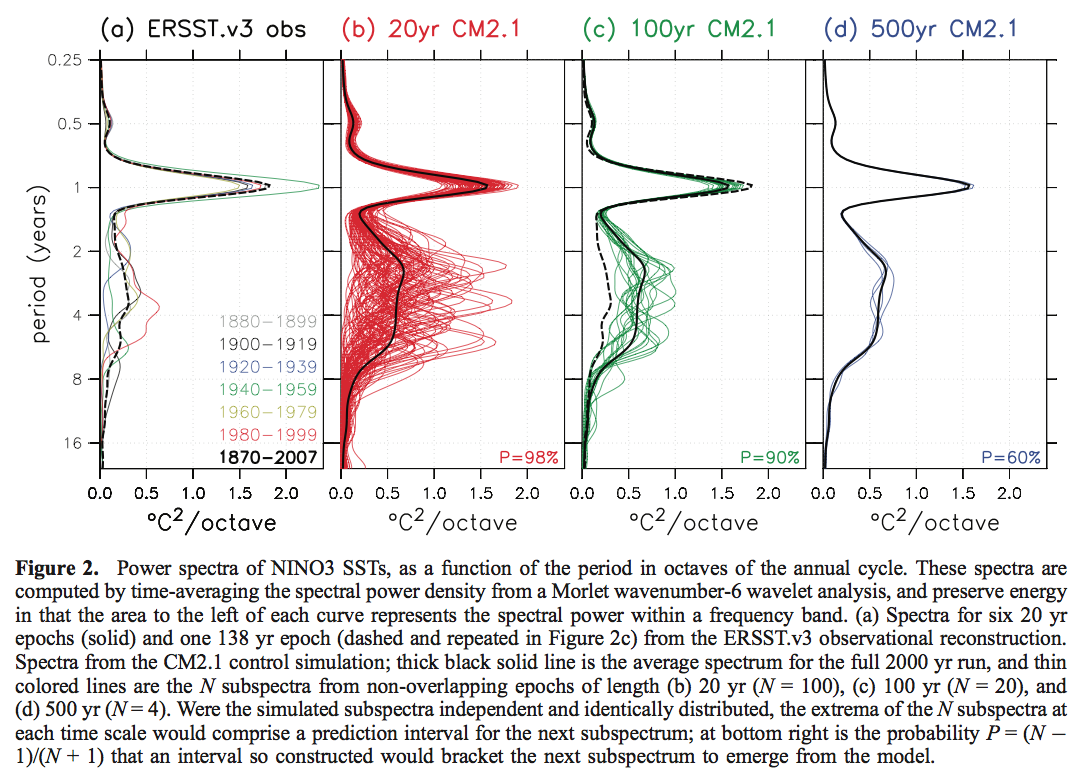
From Wittenberg 2009
Figure 2 – Click to Expand
The first graph, 2a:
..time-mean spectra of the observations for epochs of length 20 yr – roughly the duration of observations from satellites and the Tropical Atmosphere Ocean (TAO) buoy array. The spectral power is fairly evenly divided between the seasonal cycle and the interannual ENSO band, the latter spanning a broad range of time scales between 1.3 to 8 yr.
So the different colored lines indicate the spectral power for each period. The black dashed line is the observed spectral power over the 140 year (observational) period. This dashed line is repeated in figure 2c.
The second graph, 2b shows the modeled results if we break up the 2000 years into 100 x 20-year periods.
The third graph, 2c, shows the modeled results broken up into 100 year periods. The probability number in the bottom right, 90%, is the likelihood of observations falling outside the range of the model results – if “the simulated subspectra independent and identically distributed.. at bottom right is the probability that an interval so constructed would bracket the next subspectrum to emerge from the model.”
So what this says, paraphrasing and over-simplifying: “we are 90% sure that the observations can’t be explained by the models”.
Of course, this independent and identically distributed assumption is not valid, but as we will hopefully get onto many articles further in this series, most of these statistical assumptions – stationary, gaussian, AR1 – are problematic for real world non-linear systems.
To be clear, the paper’s author is demonstrating a problem in such a statistical approach.
Conclusion
Models are not reality. This is a simulation with the GFDL model. It doesn’t mean ENSO is like this. But it might be.
The paper illustrates a problem I highlighted in Part Five – observations are only one “realization” of possible outcomes. The last century or century and a half of surface observations could be an outlier. The last 30 years of satellite data could equally be an outlier. Even if our observational periods are not an outlier and are right there on the mean or median, matching climate models to observations may still greatly under-represent natural climate variability.
Non-linear systems can demonstrate variability over much longer time-scales than the the typical period between characteristic events. We will return to this in future articles in more detail. Such systems do not have to be “chaotic” (where chaotic means that tiny changes in initial conditions cause rapidly diverging results).
What period of time is necessary to capture natural climate variability?
I will give the last word to the paper’s author:
More worryingly, if nature’s ENSO is similarly modulated, there is no guarantee that the 150 yr historical SST record is a fully representative target for model development..
..In any case, it is sobering to think that even absent any anthropogenic changes, the future of ENSO could look very different from what we have seen so far.
Articles in the Series
Natural Variability and Chaos – One – Introduction
Natural Variability and Chaos – Two – Lorenz 1963
Natural Variability and Chaos – Three – Attribution & Fingerprints
Natural Variability and Chaos – Four – The Thirty Year Myth
Natural Variability and Chaos – Five – Why Should Observations match Models?
Natural Variability and Chaos – Six – El Nino
Natural Variability and Chaos – Seven – Attribution & Fingerprints Or Shadows?
Natural Variability and Chaos – Eight – Abrupt Change
References
Are historical records sufficient to constrain ENSO simulations? Andrew T. Wittenberg, GRL (2009) – free paper
GFDL’s CM2 Global Coupled Climate Models. Part I: Formulation and Simulation Characteristics, Delworth et al, Journal of Climate, 2006 – free paper
Notes
Note 1: The paper referenced for the GFDL model is GFDL’s CM2 Global Coupled Climate Models. Part I: Formulation and Simulation Characteristics, Delworth et al, 2006:
The formulation and simulation characteristics of two new global coupled climate models developed at NOAA’s Geophysical Fluid Dynamics Laboratory (GFDL) are described.
The models were designed to simulate atmospheric and oceanic climate and variability from the diurnal time scale through multicentury climate change, given our computational constraints. In particular, an important goal was to use the same model for both experimental seasonal to interannual forecasting and the study of multicentury global climate change, and this goal has been achieved.
Two versions of the coupled model are described, called CM2.0 and CM2.1. The versions differ primarily in the dynamical core used in the atmospheric component, along with the cloud tuning and some details of the land and ocean components. For both coupled models, the resolution of the land and atmospheric components is 2° latitude x 2.5° longitude; the atmospheric model has 24 vertical levels.
The ocean resolution is 1° in latitude and longitude, with meridional resolution equatorward of 30° becoming progressively finer, such that the meridional resolution is 1/3° at the equator. There are 50 vertical levels in the ocean, with 22 evenly spaced levels within the top 220 m. The ocean component has poles over North America and Eurasia to avoid polar filtering. Neither coupled model employs flux adjustments.
The control simulations have stable, realistic climates when integrated over multiple centuries. Both models have simulations of ENSO that are substantially improved relative to previous GFDL coupled models. The CM2.0 model has been further evaluated as an ENSO forecast model and has good skill (CM2.1 has not been evaluated as an ENSO forecast model). Generally reduced temperature and salinity biases exist in CM2.1 relative to CM2.0. These reductions are associated with 1) improved simulations of surface wind stress in CM2.1 and associated changes in oceanic gyre circulations; 2) changes in cloud tuning and the land model, both of which act to increase the net surface shortwave radiation in CM2.1, thereby reducing an overall cold bias present in CM2.0; and 3) a reduction of ocean lateral viscosity in the extra- tropics in CM2.1, which reduces sea ice biases in the North Atlantic.
Both models have been used to conduct a suite of climate change simulations for the 2007 Intergovern- mental Panel on Climate Change (IPCC) assessment report and are able to simulate the main features of the observed warming of the twentieth century. The climate sensitivities of the CM2.0 and CM2.1 models are 2.9 and 3.4 K, respectively. These sensitivities are defined by coupling the atmospheric components of CM2.0 and CM2.1 to a slab ocean model and allowing the model to come into equilibrium with a doubling of atmospheric CO2. The output from a suite of integrations conducted with these models is freely available online (see http://nomads.gfdl.noaa.gov/).
There’s a brief description of the newer model version CM3.0 on the GFDL page.


Your direct link to the full paper of Wittenberg does not work. It’s perhaps best to go through this link to the abstract. (or this link to the full paper)
Your direct link to the full paper of Wittenberg does not work. It’s perhaps best to go through this link to the abstract. (or this link to the full paper)
(This comment corrects a typing error in a link of my previous comment).
Thanks Pekka. I also just got an email from the paper’s author and he pointed out the same problem and gave me a better link to the full paper. I have updated the article.
I’d really like to see the calculated AMO and PDO indices from that 2,000 year run.
DeWitt,
Andrew commented:
I am going to start digging through this myself.
Thanks. I was particularly interested in the paper Predicting a Decadal Shift in North Atlantic Climate Variability Using the GFDL Forecast System because that’s the first mention I’ve seen (not that I’ve looked) in the literature about the abrupt warming of the North Atlantic Subpolar Gyre in the mid-1990’s. It stands out like a sore thumb, IMO, in the UAH NoPol anomaly time series.
My interpretation of their conclusions is that very long periods are needed to determine reliably and accurately enough statistical properties of variability as irregular as ENSO even when no long term autocorrelations exist.
People (both scientists and skeptics) tend to be too eager to draw conclusions from the history time series.
As usual, SOD, very fine post. I am always eager to learn about the time periods that are relevant for nonlinear systems, whether chaotic or not.
‘… shows 2000 years of El Nino behaviour simulated by a state-of-the-art climate model forced with present day solar irradiance and greenhouse gas concentrations. The richness of the El Nino behaviour, decade by decade and century by century, testifies to the fundamentally chaotic nature of the system that we are attempting to predict. It challenges the way in which we evaluate models and emphasizes the importance of continuing to focus on observing and understanding processes and phenomena in the climate system. It is also a classic demonstration of the need for ensemble prediction systems on all time scales in order to sample the range of possible outcomes that even the real world could produce. Nothing is certain.’ http://rsta.royalsocietypublishing.org/content/roypta/369/1956/4751.full
ENSO proxies are very revealing.
‘ENSO causes climate extremes across and beyond the Pacific basin; however, evidence of ENSO at high southern latitudes is generally restricted to the South Pacific and West Antarctica. Here, the authors report a statistically significant link between ENSO and sea salt deposition during summer from the Law Dome (LD) ice core in East Antarctica. ENSO-related atmospheric anomalies from the central-western equatorial Pacific (CWEP) propagate to the South Pacific and the circumpolar high latitudes. These anomalies modulate high-latitude zonal winds, with El Niño (La Niña) conditions causing reduced (enhanced) zonal wind speeds and subsequent reduced (enhanced) summer sea salt deposition at LD. Over the last 1010 yr, the LD summer sea salt (LDSSS) record has exhibited two below-average (El Niño–like) epochs, 1000–1260 ad and 1920–2009 ad, and a longer above-average (La Niña–like) epoch from 1260 to 1860 ad. Spectral analysis shows the below-average epochs are associated with enhanced ENSO-like variability around 2–5 yr, while the above-average epoch is associated more with variability around 6–7 yr. The LDSSS record is also significantly correlated with annual rainfall in eastern mainland Australia. While the correlation displays decadal-scale variability similar to changes in the interdecadal Pacific oscillation (IPO), the LDSSS record suggests rainfall in the modern instrumental era (1910–2009 ad) is below the long-term average. In addition, recent rainfall declines in some regions of eastern and southeastern Australia appear to be mirrored by a downward trend in the LDSSS record, suggesting current rainfall regimes are unusual though not unknown over the last millennium.’ http://journals.ametsoc.org/doi/abs/10.1175/JCLI-D-12-00003.1
Moy et al (2002) present the record of sedimentation shown above which is strongly influenced by ENSO variability. It is based on the presence of greater and less red sediment in a lake core. More sedimentation is associated with El Niño. It has continuous high resolution coverage over 12,000 years. It shows periods of high and low ENSO activity alternating with a period of about 2,000 years. There was a shift from La Niña dominance to El Niño dominance some 5,000 years ago that was identified by Tsonis (2009) as a chaotic bifurcation – and is associated with the drying of the Sahel. There is a period around 3,500 years ago of high ENSO activity associated with the demise of the Minoan civilisation (Tsonis et al, 2010). Red intensity was in excess of 200 – compare with the 1997/98 value of 98.
Of course it shows that natural variability far exceeds anything seen in the 20th century. El Niño led to globally warm conditions – it is natural to wonder how much dominant El Niño conditions in the 20th century contributed to warming – and how likely that is to turn around.
It’s even more interesting to merge that graph with Fig 1D from Marcott et al, “A Reconstruction of Regional and Global Temperature for the Past 11,300 Years”, http://content.csbs.utah.edu/~mli/Economics%207004/Marcott_Global%20Temperature%20Reconstructed.pdf , and see how much correlation there is between the red intensity and GAT. Try it.
Here’s the merged graph.
That didn’t work. Let’s try again. It may show twice. [img]”http://postimg.org/image/tk0d27k3h/”[/img]
Hmm. I used <<img src="url">, but it didn't work. SoD?
Here is Meow’s graph:
Images in comments aren’t allowed. Only authors have that privilege. You can only make links: Graph
I tried, using the url, but it didn’t work for me. Then I saved the image and uploaded it into this site and used that url and it worked.
But I see that others, including Rob Ellison made it work.. and checking, his are also wordpress graphs (another wordpress site).
It’s a recent change in WordPress that showing images in comments is possible, but that may depend on site settings. What works on many sites is including a link to the image in the comment without any tags like <img> or any other additions.
Just start a line with http and end the link with .jpg or .png that tells the type of the file. That’s likely to work.
On many sites you can right click and copy the image url. The image will show with a valid url and an image tag – png, jpeg, gif.
e.g.http://www.kingislandrenewableenergy.com.au/sites/all/files/kireip/imagecache/hero_landscape/images/hero/what_is_a_hybrid_off-grid_power_system/powerstation_king_island.jpg
If you put the address on a line by itself – as simple as that.
Others I simply snip from scientific articles usually and upload to an image library on wordpress.
I asked the paper’s author about the fraction of GFDL and NOAA’s computing resource (the 60 processors) that this simulation consumed.
Andrew replied:
That’s an interest response. What we find in our environment is that computing gets a lot faster, but customers just continue running more and more simulations with better resolution. My experience is that estimates of what adequate grid resolution is are always wrong on the low side and their estimates of how accurate and valuable the simulations are going to be are always too high. There is a certain self-selection going on here. The customers who believe in simulations are the ones who tend to run them the most and thus become the power players in the computing customer community. So there is a symbiotic relationship between those in the computer business and those in the simulation business.
Further helpful comments from Andrew Wittenberg:
I was already reading the first link above: ENSO Modulation: Is It Decadally Predictable?, Wittenberg, Rosati, Delworth, Vecchi & Zeng (2014) – it’s a fascinating paper.
SoD – thanks for looking into this, this is a great example of using a model to understand a complex system better, exactly what I was asking for in the earlier thread on 30 year averaging. Looking at the papers on observed change and proxies there seem to be clear indicators of changes in ENSO statistics on time-scales of centuries, but it seems impossible to tell if that is due to intrinsic variability or some change in forcing parameters. With a model that is close enough to reality to reproduce the essential elements of something like ENSO, you can control all those external parameters, as they did in this case, and just watch it for whatever internal behavior it does exhibit. And there is very clear evidence from this modeling of multi-decadal and century-scale variability intrinsic to the ENSO system. It might be nice to understand that better, but there may be no easy way to do that – the recent paper reports testing with slightly varied starting conditions and seeing weak ENSO periods become strong, so it does seem this is really intrinsic chaotic behavior, not the manifestation of some other system that has a long-term memory.
So – well done, and I think this is pretty clear evidence (assuming other model simulations agree) for intrinsic multi-decadal variability.
[…] « Natural Variability and Chaos – Six – El Nino […]
And see also this comment from A Pacific Centennial Oscillation Predicted by Coupled GCMs, Karnauskas et al (2012).
It is clear that ENSO is influenced by the strong periodicity of the QBO. It is likely much more periodic than chaotic.
[…] a comparison on resolution, the 2,000 year El Nino study we saw in Part Six of this series had an atmospheric resolution of 2.5º x 2.0º with 24 […]
The authors wrote: “More worryingly, if nature’s ENSO is similarly modulated, there is no guarantee that the 150 yr historical SST record is a fully representative target for model development.”
I love (sarcasm intended) seeing modelers question the existence of reality – the historical record. However, their data shows that 100 years of historical record is marginally adequate – assuming we can trust the limited historical record before El Nino was a recognized and well-observed phenomena.
BEFORE questioning the usefulness of the historical record, however, we should ask whether models are capable of reconstructing the reality of ENSO. Is the model fit for the purpose for which it is being used? Neither the author nor SOD bothered to address this question.
To begin with, no model in existence is currently capable of predicting the state of ENSO even one year in the future when initialized with the best observational data we have.
Models do a poor job of reproducing phenomena important to ENSO. For example, climate models don’t accurately reproduce the MJO or Kelvin waves.
http://journals.ametsoc.org/doi/full/10.1175/2009JCLI3422.1
http://journals.ametsoc.org/doi/abs/10.1175/JCLI-D-12-00541.1
Most CMIP5 models produce a split ITCZ.
FInally, let’s consider the full uncertainty inherent in this model and think about an ensemble of perturbed-parameter GFDL models. What will that do to the NINO3 SST power spectrum?
SOD was clearly thinking about the right question when he wrote: “Models are not reality. This is a simulation with the GFDL model. It doesn’t mean ENSO is like this. But it might be.” In the case of ENSO, “it might be” seems to be overly generous.
I don’t object to SOD questioning the usefulness of the historical record – it is a single realization of a chaotic system. I do question whether climate models are capable of providing a useful answer to this problem.