Feeds:
Posts
Comments

Archive for March, 2011

In this article in the series we will look an interesting paper:

An analysis of the dependence of clear-sky top-of-atmosphere outgoing longwave radiation on atmospheric temperature and water vapor, by Dessler, Yang, Lee, Solbrig, Zhang and Minschwaner, JGR (2008).

This paper can be downloaded for free.

I used some results of this paper in Theory and Experiment – Atmospheric Radiation, but only for comparing calculated top of atmosphere radiative fluxes vs measurement.

I think that the “basic physics” of radiative transfer and atmospheric convection is challenging enough, and the question of feedback even harder.

There are hundreds of papers (thousands really) on this confusing subject and so, for me, drawing conclusions requires a lot of research. Luckily, most people interested in the climate debate already know the answer to the question of feedback from water vapor, so this article won’t be so interesting to them.

In fact, the paper under review doesn’t claim any real answers in the subject of water vapor feedback with climate change:

We are looking at regional variations in lapse rate in a fixed climate, rather than variations in the average lapse rate as the climate changes. This result demonstrates the unsuitability of using variations in different regions in our present climate as a proxy for climate change.

But even with the guarded comments of a published paper, the results are very interesting – and help, at the very least, to illuminate some aspects of how water vapor and atmospheric temperature interact to change the radiative cooling from the planet.

So for people looking for a quick answer, it’s not here. For people wanting to understand the interaction between surface temperature, atmospheric temperature, water vapor and outgoing longwave radiation (OLR) – this might provide a few insights on their journey.

Background

In trying to understand feedback we want to know what happens to the outgoing longwave radiation (OLR) from the climate as surface temperature changes.

Some basic (but hard to calculate) radiative physics – already covered in many places including CO2 – An Insignificant Trace Gas? Part Seven – The Boring Numbers (and the preceding parts of the series) – tells us that, all other things being equal, a doubling of CO2 in the atmosphere from pre-industrial levels will lead to a surface temperature change of about 1°C.

Apart from other variability – how will the climate respond to this increase in surface temperature?

It is only by isolating different causes and effects that we can hope to understand the complexity of the climate. It’s slow but there is more chance of getting the correct answer.

The main miscreant identified as possibly causing a much higher than 1°C increase is water vapor feedback. Water vapor is the dominant “greenhouse” gas, but is variable in space and time as it responds to climate conditions. See, for example, Clouds and Water Vapor – Part Two.

When we think about feedback, one of the most important considerations is how OLR responds to a change in surface temperature.

Let’s consider the change in surface radiation when the temperature increases by 1°C. Most of the earth’s surface has an emissivity very close to 1. At 15°C the increase in surface radiation for this 1°C increase, ΔR = 5.5 W/m². So if the OLR also increased by 5.5 W/m² then the feedback from the climate would be zero. (See comment below for why this is not quite correct).

Why? Because all of the increase in surface radiation has also been emitted from the climate system into space. Picture the scene if instead 10 W/m² was emitted into space after this 1°C increase in surface temperature – this would be negative feedback.

And if the OLR change was 1 W/m² ? This would be positive feedback. Because the increase in radiation from the surface wasn’t matched by radiation from the climate system.

If this doesn’t make sense, ask a question. It’s hard to make progress without grasping this point.

Measurements and “Model”

Dessler compares the results of over 100,000 measurements of top of atmosphere (TOA) fluxes from the CERES satellite with two band models which provide computational efficiency (see note 1).
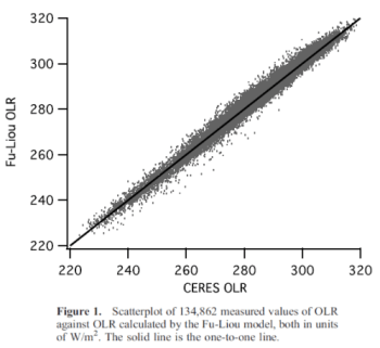
Figure 1 – Comparison of a band model with measured results

This is simply to demonstrate that the model for calculating TOA fluxes is reliable and accurate. The results are used for later calculations. Other graphs in the paper compare the results against surface temperature and latitude to confirm that no bias exists in the results.

Atmospheric temperature and water vapor are measured using AIRS – Atmospheric Infrared Sounder flying on the NASA Aqua satellite. CERES = “Clouds and the Earth Radiant Energy System”, which is also flying on the Aqua satellite.

The measurements taken by AIRS and CERES are “virtually simultaneous”.

These measurements were all taken in March 2005 between 70°N and 70°S over the ocean under clear skies.

The measurements were selected from nighttime measurements. Why? To eliminate any contribution around the 4μm wavelength from solar radiation.

A Basic Equation

Equations aren’t fun for a lot of people and that’s understandable. Stay with me, I will try and explain it in plain English.

What we want to know is how OLR (radiation from the climate to space) changes as surface temperature changes. If we can establish this, we can understand how the climate currently responds to surface temperatures – and what feedbacks are currently in place, at least for the time under consideration:

Figure 2 – The equation

The red term is the main value we want to know – the “rate of change” of OLR with surface temperature

Or, how much does the outgoing longwave radiation change as surface temperature changes?

The orange term = the sum (vertically through the atmosphere) of all the changes in OLR as surface temperature changes, due to the change in atmospheric temperature

The green term = the sum (vertically through the atmosphere) of all the changes in OLR as surface temperature changes, due to the change in water vapor

And before we “dive in”, the basic concepts are, in simple terms:

  • if the atmosphere gets warmer it radiates more to space – and this cools the climate
  • if water vapor increases it reduces the OLR (because it is a “greenhouse” gas) – and this heats the climate (because less radiation to space takes place)
  • if water vapor increases it reduces the “lapse rate” (note 2), making the atmosphere warmer higher up, increasing radiation to space – and this cools the climate

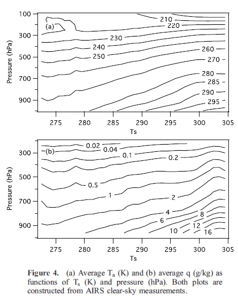
Now let’s take a look at the graphical picture of how atmospheric temperature and humidity vary with surface temperature and height. Think of surface temperature as a proxy for latitude.

Here is how the air temperature vs height, and humidity vs height, vary with surface temperature:

from Dessler (2008)

Figure 3 – Measurements

For those new to humidity measurements in the atmosphere, note the strong dependency on surface temperature and on height in the atmosphere (1000hPa is the surface and 200hPa is around 12km above the surface).

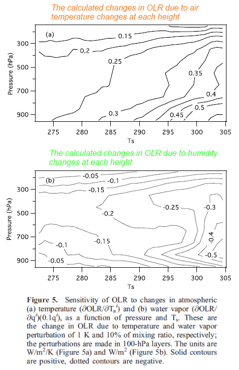
Now we want to plot two of the terms in the equation (figure 2). The colors are matched up with the highlighted terms in the original equation.

From Dessler (2008)

Figure 4 – Calculated – Color text added

These values are calculated by using the model. (We have already seen that this band model accurately calculates the OLR from surface temperature, air temperature and humidity).

As you would expect, when air temperature increases by 1K the OLR increases – because a hotter atmosphere radiates at a higher intensity. This is with all other conditions held the same.

And as you might expect, when the humidity is increased by 10% the OLR decreases – because a more opaque atmosphere has a lower transmittance to surface radiation. This is with all other conditions held the same.

We have been calculating these terms from figure 2:

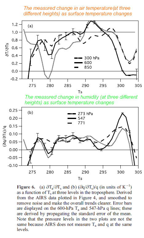
Now, find how OLR changes due to surface temperature changes we need to also find out these terms:

Or, in English:

  • the change in air temperature due to surface temperature changes
  • the change in humidity due to surface temperature changes.

From Dessler (2008)

Figure 5 – Measured – Color text added

So, to give an example of what these graphs show, we can see that at around 293-294K, an increase in surface temperature has little or no effect on humidity. Around 300K an increase in surface temperature has a large effect on humidity.

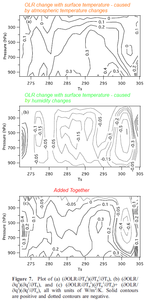
Now we are going to multiply the terms together to find:

  • the change in OLR with surface temperature – due to atmospheric temperature changes
  • the change in OLR with surface temperature – due to humidity changes

Figure 6 – Results – Color text added

The advantage of this method is that when we look at the summary and say, for example:

Oh that’s interesting, the strongest positive feedback effects are around 302 K, what causes that? The strongest negative feedback effects are around 290 – 295 K, what causes that?

– we can review the terms that created the result and see which dominates – and why.

Looking at the total, we can see that between 298 – 303 K the OLR decreases as surface temperature increases (note that the plot is of the change in OLR as Ts increases versus Ts). And below 298 K the OLR increases as surface temperature increases.

This is in agreement with Raval & Ramanathan’s work based on ERBE data shown in Part One where the positive feedback comes from the tropics, and is reduced by the negative feedback from the sub-tropics and mid-latitudes.

The decrease of OLR as surface temperature increases became known as the super-greenhouse effect. Remember that any effect below an increase of 5.5W/m².K (at 15°C) is a positive feedback. (And at 30°C, this threshold value is 6.3W/m².K). An actual decrease of OLR as surface temperature increases is, therefore, a very strong positive feedback effect.

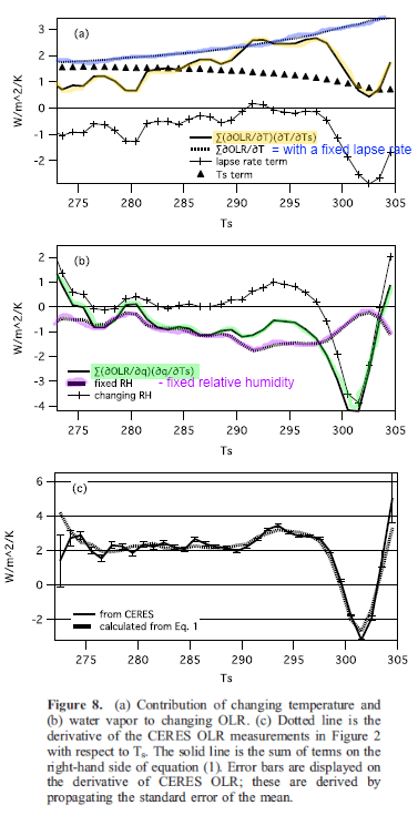
We can see the result plotted against surface temperature and height – now let’s see the total value against surface temperature, and some comparisons of the actuals vs reference scenarios:

Figure 7 – Color text and highlighting added

The first graph shows the change in OLR with surface temperature – due to atmospheric temperature changes. The blue line shows the result if the lapse rate was fixed. Remember that a lower value of changing OLR with Ts is more towards positive feedback.

This is a quantitative estimate of the effect of the changing lapse rate on dOLR/dTs, and it shows that it is negative for almost all values of Ts. In other words, as Ts increases, so does the lapse rate, and the general effect of this is to reduce dOLR/dTs, and therefore OLR, below what they would be if the atmosphere maintained a constant lapse rate.

The second graph shows the change in OLR with surface temperature – due to humidity changes. The purple line shows the result if relative humidity was constant. (And see the results from Sun & Oort, shown in Part Three).

In the subtropics, the ‘‘changing RH’’ line is positive, meaning that RH decreases with increasing Ts. This relative dryness contributes to high values of OLR here, providing a key pathway for the climate system to lose energy back to space. As Ts crosses the convective threshold, ≈298 K, the RH of the atmosphere abruptly increases, leading to a strong increase in q and a reduction in OLR and its gradient.

The third graph compares the results by using the data graphed in Figure 1 with the results derived through this article – and they are the same.

We also plot in this panel the right-hand side of equation (1):

Σi(∂OLR/∂Ti)(∂Ti/∂Ts) + Σi(∂OLR/∂qi)(∂qi/∂Ts) + ∂OLR/∂Ts,

derived from lines plotted in Figures 8a and 8b. As one can clearly see, the agreement is excellent. Note that this is a stringent test as these two lines are derived from completely independent data: one line is derived entirely from CERES data while the other line is derived entirely from AIRS data and a radiative transfer model. The excellent agreement gives us great confidence that, given observations of Ta and q, the clear-sky OLR budget is well understood inthe present atmosphere. We also see no evidence that neglected terms are important, in agreement with previous work..

Conclusion

The paper gives us an excellent insight into how atmospheric temperature and humidity vary as surface temperature varies – over the ocean. And how this maps into changes in OLR as surface temperature changes.

We see that the results are similar to Ramanathan’s work shown in Part One.

These are valuable insights.

If surface temperature increases from any cause, does this mean that positive feedback from water vapor will amplify this? If surface temperature reduces from any cause, does this mean that positive feedback from water vapor will amplify this?

Surely that depends.

But ask yourself this – if the results had shown the opposite effect, would you find them significant?

Articles in this Series

Part One – introducing some ideas from Ramanathan from ERBE 1985 – 1989 results

Part One – Responses – answering some questions about Part One

Part Two – some introductory ideas about water vapor including measurements

Part Three – effects of water vapor at different heights (non-linearity issues), problems of the 3d motion of air in the water vapor problem and some calculations over a few decades

Part Five – Back of the envelope calcs from Pierrehumbert – focusing on a 1995 paper by Pierrehumbert to show some basics about circulation within the tropics and how the drier subsiding regions of the circulation contribute to cooling the tropics

Part Six – Nonlinearity and Dry Atmospheres – demonstrating that different distributions of water vapor yet with the same mean can result in different radiation to space, and how this is important for drier regions like the sub-tropics

Part Seven – Upper Tropospheric Models & Measurement – recent measurements from AIRS showing upper tropospheric water vapor increases with surface temperature

Notes

Note 1: See CO2 – An Insignificant Trace Gas? Part Four for more explanation of “band models”. A “model” doesn’t mean “GCM”. In this case it simply means a more efficient way of calculating the TOA flux than using “line by line” calculations in the radiative transfer equations.

The HITRANS database contains 2.7M spectral lines and so “doing it the long way” takes a lot of time. Therefore, over time, many band models have been created – and critically evaluated – against the hard way.

Note 2: The lapse rate is the decrease in temperature as you go up through the atmosphere. In a dry atmosphere the temperature reduces at around 10K/km. In a very moist atmosphere the temperature reduces at around 4K/km. And, on average, the lapse rate is 6.5K/km. So the more water vapor there is in the atmosphere, the warmer the atmosphere at any given height.

Read Full Post »

In the last article we looked at some results from Grant Petty.

In essence they demonstrate the huge variation in the transmittance of CO2 through the atmosphere with the wavelength of radiation.

I decided it might be interesting to try and reproduce these results using the HITRAN database. This allows a closer examination of which mechanisms cause which results.

Line Shapes and Pressure Broadening

The energy in a photon is given by a very simple equation:

E = hν

where h = Planck’s constant = 6.63 x 10⁻³⁴ J.s, and ν = frequency (ν=c/λ where c=speed of light and λ = wavelength)

So, for example, a 15μm photon has an energy of 1.3 x 10⁻²⁰ J.

A photon can be absorbed by a molecule if the energy of the photon matches the exact energy required to change the state of that molecule.

Now, if a photon was only absorbed at one exact wavelength then atmospheric radiation would be irrelevant.

An easy concept for people who have done a lot of maths or physics, but not so obvious to many others.

Let’s take a different example. If you start your car up and accelerate steadily up to 60 miles per hour over 1 minute, how long do you spend at the speed of 34.5698895549034592345123 miles per hour? Not much. And the more precise I make this speed, the less time you will have spent at it.

If we consider how much energy is transferred in terrestrial radiation from the surface at 14.995698895549034592345123 μm, the answer is “not much”. The same goes for any other vanishingly small interval of wavelengths.

So if each absorption line was exactly one wavelength then the amount of energy absorbed by a finite number of lines would be zero.

However, each absorption line has a finite width. Part of this is due to the uncertainty principle described by quantum mechanics – the small time a higher energy state is occupied produces an uncertainty in the energy of that state.

This is called natural broadening and is a very small effect.

The easiest broadening mechanism to understand is Doppler broadening. Molecules in the atmosphere are zipping around in all directions at speeds of around 500 m/s. Compared with the speed of light this is small, but the difference in the relative speed between a photon and a molecule is slightly changed, leading to a change in the absorption frequency (see note 1 for more details). This is “relatively easy” to understand from first principles and the mathematical treatment is straightforward.

The dominant line broadening mechanism in the lower atmosphere is pressure, or collisional, broadening. This is more challenging from a theoretical point of view but is certainly a measurable value.

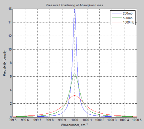
The main effect of pressure broadening is to “spread out” the absorption line. Here is a typical example, where 1000mb is at the earth’s surface, and 200mb is at the “tropopause”, or top of the lower atmosphere:

Figure 1

So the absorption at the center of the line is reduced, while more absorption takes place out to the sides.

The parameter which describes how much broadening has taken place is called the half-width – and is the width of the line when the value has dropped to half the peak value.

Typical values of pressure broadening half width are 0.01 – 0.1 cm-1 at 296 K and pressure of 1000 mb (surface atmospheric pressure).

The function which approximates this effect is the Lorentz line shape:

f(ν-ν0) = αL/π((ν-ν0)²+αL²)       [1]

where ν0 is the frequency of the absorption, ν = frequency and αL = half-width at half of the maximum

And the half-width at any given temperature and pressure is given by this formula:

αL = α0(p/p0).(T0/T)γ [2]
where α0 = lab measured half-width at pressure p0 and temperature T0, and γ is also a lab measured parameter, typically around 0.5 – 0.7.

That’s a lot to take in if you haven’t seen it before. Take a look back at Figure 1 – this is what these formulas describe.

The atmospheric pressure where pressure broadening is comparable to Doppler broadening is about 10 mbar. This is around 30km above the surface, so in the troposphere Doppler broadening is unimportant.

In a later article we might explore the experimental results vs theoretical results of pressure broadening in more detail. Or at least, how much inaccuracies might affect radiative transfer calculations.

HITRAN database

You can read more about the HITRAN database here. The most recent update of the database is described in The HITRAN 2008 molecular spectroscopic database, by L.S. Rothman et al, and the earlier 2004 update: The HITRAN 2004 molecular spectroscopic database, by L.S. Rothman et al.

This database is the result of a huge amount of work by thousands of researchers over a few decades. If you look at the references in the 2008 paper you find almost 400 papers.

In the previous articles in this series I created two fictitious molecules, pCO2 and pH20, and solved the radiative transfer equations for a variety of conditions for these two molecules through the atmosphere.

The aim of this simplification was illumination.

Given that the HITRAN database contains over 300,000 absorption lines for CO2 (and 2.7M lines in total), I thought that replicating some standard results (e.g. see Part Eight) might be a little too much of a challenge. However, the hardest part was actually reading the database, which is in text form – and the problems were just due to my novice status with MATLAB.

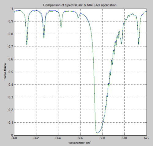
DeWitt Payne kindly offered me some results he obtained from SpectralCalc (via subscription). These were from 660-672 cm-1 through a 1 meter path at standard temperature and pressure, and CO2 concentrations of 380 ppm.

Here is the comparison with my MATLAB program:

Figure 2

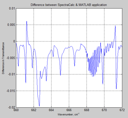
And here is the difference between the two results (the SpectralCalc results minus the MATLAB results):

Figure 3

The MATLAB program, for the results above, only considered the main isotopologue of CO2, which accounts for over 98% of the concentration of CO2 in the atmosphere. However, including the absorption lines for all isotopologues had almost no effect and the small differences remain.

As the differences are small, it seems worth showing some initial results from the program.

Results

First, let’s see the effect of “pressure broadening”.

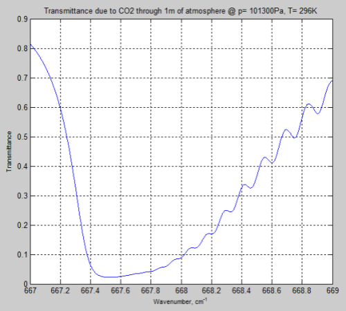
Here is the result through 1m of atmosphere at the earth’s surface, around the peak absorption wavenumber of CO2:

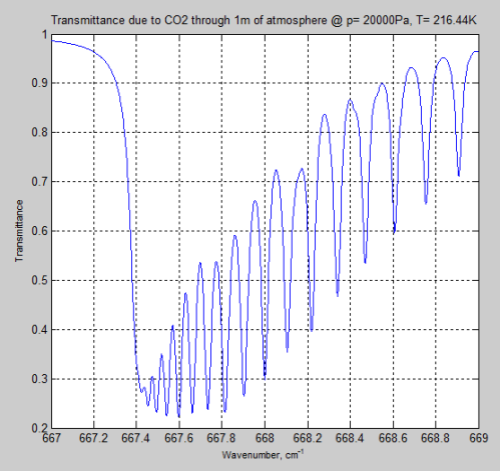
Figure 4

And the result for the same 1m of atmosphere at the tropopause (top of the troposphere) at 200mbar (typically around 12km):

Figure 5

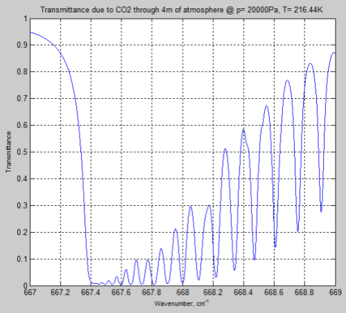
Now at 200 mbar there is less atmosphere so the comparison isn’t truly a fair one. Increasing the path length to get the same number of CO2 molecules we get this result:

Figure 6

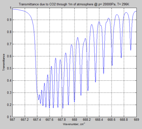
Both pressure and temperature have changed so it’s worth seeing the result if we apply the surface temperature to the Figure 5 results:

Figure 7

We can see from the result (and it’s also clear from the equations earlier) that the parameter having the most effect is the pressure – which changes by a factor of 5. The temperature reduction from 296K to 216K has a much smaller impact.

However, the difference between Figure 4 and Figure 6 is very significant – individual lines are “smeared out” at the earth’s surface, but distinct lines higher up in the atmosphere.

Let’s take a look at a wider range of wavenumbers / wavelengths.

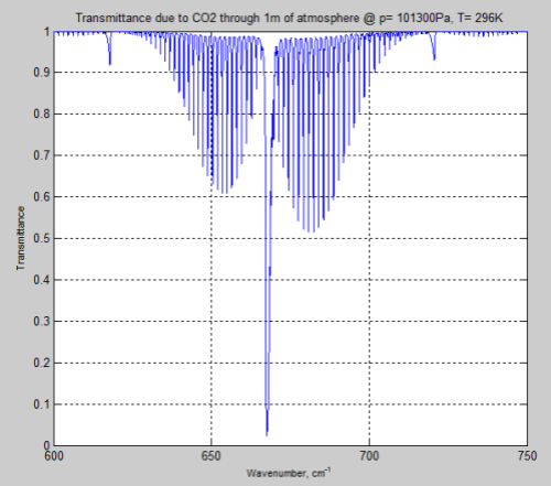
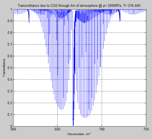
From 600 – 750 cm-1 (13.3 – 16.7 μm) at the surface through 1 meter of atmosphere:

Figure 8

And the same amount of CO2 at the tropopause:

Figure 9

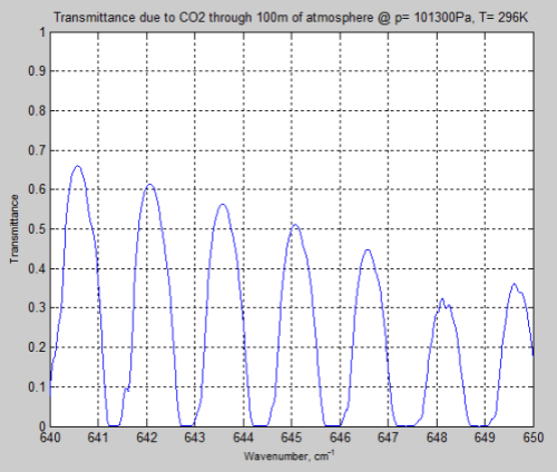
Let’s look at a longer path of 100m through the atmosphere and “zero in” on one part of the bandwidth, 640-650 cm-1:

Figure 10

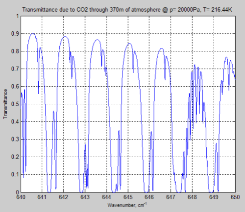
And let’s compare it with the tropopause, again through a longer path, to keep the CO2 quantity the same:

Figure 11

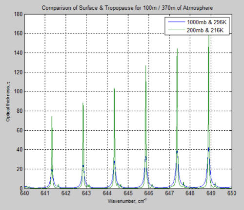
Just for interest I compared the optical thickness of the surface and tropopause for these wavenumbers on the same graph. Optical thickness increases as transmittance decreases. Check out the heading Optical Thickness & Transmittance in Part Six if this isn’t clear.

Figure 12

We can see that the peaks of absorption are indeed lower but the widths of the absorption lines are wider (for the surface results).

Saturation Revisited

As I commented in Part Eight, many people have heard about the high absorption of CO2 at 15 μm and have not understood the huge variation in absorption across the wide bandwidth of CO2. (Also there is the most important subject of re-emission).

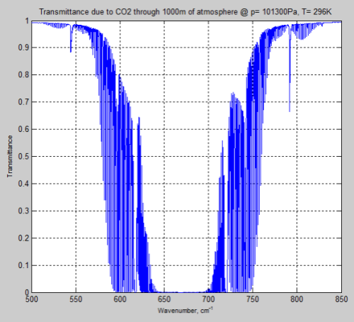
Here is the result of the simple “slab” model, which calculates the transmittance through 1km of atmosphere (a slab model means that the pressure and temperature are constant through the “slab” – a very simple model):

Figure 13

As you can see, around 570 – 600 cm-1 (16.7 – 17.5 μm) and 730 – 770 cm-1 (13.0 – 13.7 μm) the transmittance through the atmosphere is nowhere near “saturated”.

If 1 km of atmosphere has a transmittance of 0.7 (i.e., 70% of radiation is transmitted) at some wavelengths then clearly more CO2 will reduce this transmittance.

The Matlab Code

The results were all created using my code: HITRAN_0_2. However, each run has slightly different parameters, which are adjusted by changing the code rather than anything more elegant. See Note 2 for the code.

The code at this stage has provision for different layers of different temperatures, pressures, and densities – but at this stage the code doesn’t use it – just one “slab”.

The core part of the code is very simple:

  • Take each absorption line in turn and use its measured line strength, half width, and other parameters
  • For the pressure and temperature, calculate the half width for those conditions (equation 2)
  • Now for each line, take each wavenumber in turn (defined via a start, stop and interval) and apply the formula in equation 1 to calculate the optical thickness
  • Add the optical thickness at this wavenumber to the optical thickness already calculated for this wavenumber

The code could be more “speed efficient” – by only calculating equation 1 close to the absorption line. I started out simpler to see what happened and it went so fast that I didn’t improve it.

Multiple Atmospheric Layers

As the pressure and temperature change with height through the atmosphere the single slab model is limited in value.

So I extended the model to multiple layers – v0.3 (see Note 2).

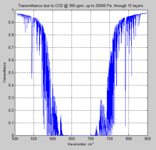
Here is the result of transmittance up to 200mb (20,000 Pa) from CO2 at 360 ppm with a 15 layer model:

Figure 14

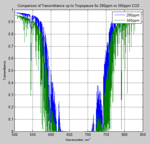
And, of course, the question many people have – what is the difference between the atmosphere at 280 ppm and 560 ppm – or a doubling of CO2 from pre-industrial levels:

Figure 15

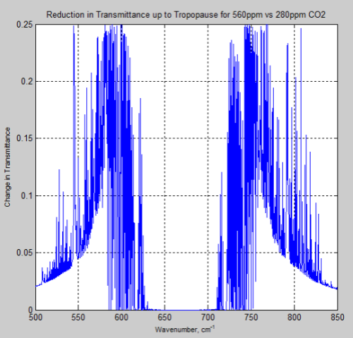
And the difference between the two, the “delta”:

Figure 16

Remember – or note, if this is new – the atmosphere absorbs and also re-emits. The question of radiative forcing cannot be answered by only considering transmittance.

However, these graphs of the change should at least indicate to people that the issue of the very high optical thickness = very low transmittance at 667 cm-1 = 15 μm is not the complete story, even only considering transmittance.

Limitations

The model has the limitation at the moment that it doesn’t take into account Doppler broadening. If we extend the model up into the stratosphere Doppler broadening starts to become important. I might get around to including this by introducing the Voigt function which combines pressure broadening and Doppler broadening.

There is also the possibility that my model has a mistake. However, I have compared it to the results from SpectralCalc and it is very close, and to results published in Grant Petty’s book, which look the same.

Other articles:

Part One – a bit of a re-introduction to the subject.

Part Two – introducing a simple model, with molecules pH2O and pCO2 to demonstrate some basic effects in the atmosphere. This part – absorption only.

Part Three – the simple model extended to emission and absorption, showing what a difference an emitting atmosphere makes. Also very easy to see that the “IPCC logarithmic graph” is not at odds with the Beer-Lambert law.

Part Four – the effect of changing lapse rates (atmospheric temperature profile) and of overlapping the pH2O and pCO2 bands. Why surface radiation is not a mirror image of top of atmosphere radiation.

Part Five – a bit of a wrap up so far as well as an explanation of how the stratospheric temperature profile can affect “saturation”

Part Six – The Equations – the equations of radiative transfer including the plane parallel assumption and it’s nothing to do with blackbodies

Part Seven – changing the shape of the pCO2 band to see how it affects “saturation” – the wings of the band pick up the slack, in a manner of speaking

Part Eight – interesting actual absorption values of CO2 in the atmosphere from Grant Petty’s book

Part Nine – calculations of CO2 transmittance vs wavelength in the atmosphere using the 300,000 absorption lines from the HITRAN database

Part Ten – spectral measurements of radiation from the surface looking up, and from 20km up looking down, in a variety of locations, along with explanations of the characteristics

Part Eleven – Heating Rates – the heating and cooling effect of different “greenhouse” gases at different heights in the atmosphere

Part Twelve – The Curve of Growth – how absorptance increases as path length (or mass of molecules in the path) increases, and how much effect is from the “far wings” of the individual CO2 lines compared with the weaker CO2 lines

And Also –

Theory and Experiment – Atmospheric Radiation – real values of total flux and spectra compared with the theory.

References

The HITRAN 2008 molecular spectroscopic database, by L.S. Rothman et al, Journal of Quantitative Spectroscopy & Radiative Transfer (2009)

Notes

Note 1 – The energy absorbed from a photon, E = hv, where h = Planck’s constant, and ν= frequency. The energy of the photon has to match precisely the energy required for the change in state of the molecule.

However, due to the motion of atmospheric molecules, the actual frequency, ν’ = ν(1-ν/c), where c = speed of light, ν = frequency measured by a stationary observer.

In essence, there is now a very small (but measurable) range in frequencies (with respect to a “stationary” planet) that can be absorbed to give the precise energy level required for a transition of this molecule – and so the faster the molecules are moving, the more the absorption line “spreads out”.

Molecular speeds are given by the Maxwell-Boltzmann distribution.

Note 2

HITRAN v0.2

HITRAN v0.3

And the code for v0.2 reproduced here for convenience:

====== HITRAN v0.2 ===================

function [vmin vmax dv cco2 T p d vt tau ] = HITRAN_0_2()

% Absorption through atmosphere of defined temperature & pressure

% uses the HITRANS database

%

% v0.1 – Basic calculations to get out of the starting blocks

% v0.2 – Tidy up and allow a “slab” to be at any pressure and temperature

%       with line width determined by the pressure & temperature

clear

disp([‘—- New Run —- ‘ datestr(now) ‘ —-‘]);

disp(‘  ‘);

% =========== Basic definitions =====================

p0=1.013e5; % std pressure for the HITRANS database in Pa

T0=296; % std temperature for HITRANS database in K

cco2=360e-6; % concentration of CO2

Na=6.02e23; % Avogradro’s number

mair=29e-3; % molar mass of air

% now define the fractional abundance of each isotopologue of CO2

isoprop=[0.98420 0.01106 0.0039471 0.000734 0.00004434 0.00000825 0.0000039573 0.00000147];

ignoreiso=false; % allows easy switching between main isotopologue only or all of them

% =========== Define wavenumber ranges ==============

vmin=640; % min wavenumber to consider (overall)

vmax=650; % max wavenumber to consider (overall)

dv=0.001; % resolution of wavenumber

% because absorption lines below the lower boundary (and above the upper

% boundary) can still affect the wavenumbers under consideration we need to

% extend the boundaries of which absorption lines to consider

rvmin=0.98; % ratio below lower boundary to consider

rvmax=1.02; % ratio above upper boundary to consider

%vt=vmin:dv:vmax; % vt = wavenumbers we will calculate optical depth for

vt=linspace(vmin,vmax,1063);

vtmax=length(vt);

tau=zeros(1,vtmax); % set optical depth to zero as a starting point

% =========== Read in CO2 data and select vmin-vmax data ========

% selected paramaters for complete HITRAN CO2 database already stored in file: co2.mat

load(‘co2’);

if ignoreiso==true

% select only main isotopologue between the wavenumber boundaries

iv=find(iso==1 & v>vmin*rvmin & v<vmax*rvmax); % select upper and lower bounds

else

% select all isotopologues and between the wavenumber boundaries

iv=find(v>vmin*rvmin & v<vmax*rvmax); % select upper and lower bounds

end

% select subset of CO2 spectral data for evaluate

iso=iso(iv); v=v(iv); S=S(iv); gama=gama(iv); nair=nair(iv);

ivmax=length(v);

% ============= Define standard atmosphere against height ================

% reuse code from rte_0_5_0 to define std atmosphere and number of levels

% SI units used unless otherwise stated

% first a “high resolution” atmosphere

% zr = height, pr = pressure, Tr = temperature, rhor = density

Ts=296; % define surface temperature at same value as HITRAN measurements

ps=1.013e5; % define surface pressure

Ttropo=215; % define tropopause temperature

% nmv=2.079e25; % nmv x rho = total number of molecules per m^3, not yet

% used

maxzr=50e3; % height of atmosphere

numzr=5001; % number of points used to define real atmosphere

zr=linspace(0,maxzr,numzr); % height vector from sea level to maxzr

[pr Tr rhor ztropo] = define_atmos_0_3(zr,Ts,ps,Ttropo); % function to determine (or lookup) p, T & rho

% Create “coarser resolution” atmosphere – this reduces computation

% requirements for absorption & emission of radiation

% z, p,Tinit,rho; subset of values used for RTE calcs

numz=10; % number of boundaries to consider (number of layers = numz-1)

minp=2e4; % top of atmosphere to consider in pressure (Pa)

% want to divide the atmosphere into approximately equal pressure changes

dp=(pr(1)-minp)/(numz); % finds the pressure change for each height change

zi=zeros(1,numz); % zi = lookup vector to “select” heights, pressures etc

for i=1:numz % locate each value

zi(i)=find(pr<=(pr(1)-i*dp), 1); % gets the location in the vector where

% pressure is that value

end

% now create the vectors of coarser resolution atmosphere

% z(1) = surface; z(numz) = TOA

% T, p, rho all need to be in the midpoint between the boundaries

% T(1) is the temperature between z(1) and z(2), etc.

z=zr(zi);   % height

pb=pr(zi);   % pressure at boundaries

Tb=Tr(zi);   % starting temperature at boundaries

rhob=rhor(zi);  % density at boundaries

% now calculate density, pressure and temperature within each layer

for i=1:numz-1

dz(i)=z(i+1)-z(i); % precalculate thickness of each layer

Tinit(i)=(Tb(i+1)+Tb(i))/2; % temperature in midpoint of boundary

p(i)=(pb(i+1)+pb(i))/2; % pressure in midpoint of boundary

rho(i)=(rhob(i+1)+rhob(i))/2; % density in midpoint of boundary

end

% ===============

% but in the first version we ignore this and just calculate at std temp

% and pressure (later iterate through each layer, i

% work in cm for volumes and distances (absorption coefficients are in cm)

p=p0;

rhop=rhor(find(pr<=p,1)); % lookup density at pressure = p

T=Tr(find(pr<=p,1)); % lookup temperature at pressure = p

na=(Na*rhop/mair)/1e6; % number of air molecules per cm^3

Nco2=na*cco2; % number of CO2 molecules per cm^3

d=100*100; % path length in cm *** just a starting point

% ======== Iterate through each absorption line ======

% for one slab of depth, d

for j=1:ivmax  % each absorption line

% v(j)=line center, S(j)=line strength, gama(j)=half width

% first do a code inefficient method – calculate the profile for each

% across the entire wavenumber range

if ignoreiso==true   % if we only want to consider the main isotopologue

prop=Nco2;

else

prop=isoprop(iso(j))*Nco2;

end

ga=gama(j).*(p/p0).*(T0/T).^nair(j);

% ======== Iterate through each wavenumber  ====

for k=1:vtmax  % each wavenumber

%  vt(k) is the wavenumber under consideration

dtau=prop*d*S(j)*ga/pi/((vt(k)-v(j))^2+ga^2);

tau(k)=tau(k)+dtau;

end

end

plot(vt,exp(-tau))

title([‘Transmittance due to CO2 through ‘ num2str(round(d/100))…

‘m of atmosphere @ p= ‘ num2str(p) ‘Pa, T= ‘ num2str(T) ‘K’])

ylabel(‘Transmittance’,’FontSize’, 8)

xlabel(‘Wavenumber, cm^-^1′,’FontSize’, 8)

grid on

disp([‘Range = ‘ num2str(vmin) ‘ – ‘ num2str(vmax) ‘ cm^-1, dv = ‘ num2str(dv) ‘, lines = ‘ num2str(ivmax)]);

disp([‘Number of CO2 molecules per cm^3 = ‘ num2str(Nco2) ‘, path length = ‘ num2str(d/100) ‘ m’]);

disp([‘p= ‘ num2str(p) ‘ Pa, T= ‘ num2str(T) ‘ K’]);

disp([‘—- Complete End —- ‘ datestr(now) ‘ —-‘]);

======== end of HITRAN v0.2 =====================

Read Full Post »

I thought some data provided in Grant Petty’s excellent book would be valuable as it helps explain some important points about the role of CO2 in the atmosphere.

Just recently I was kindly given access to the HITRAN database by Dr. Laurence S. Rothman but I’ve spent a bit too much time in the last few days trying to get MATLAB to read it (still a novice at MATLAB). I do plan to provide a followup article with some calculations of my own on the HITRAN data. Who knows how long that will take.

HITRAN is an acronym for high-resolution transmission molecular absorption database. It is a treasure trove of spectroscopic data.

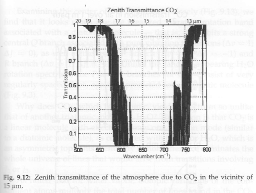
First, here’s a couple of extracts from A First Course in Atmospheric Radiation by Grant Petty. (I briefly reviewed this book in Find Stuff Out and Book Reviews):

From "A First Course in Atmospheric Radiation", Grant Petty (2006)

From "A First Course in Atmospheric Radiation", Grant Petty (2006)

What is “zenith transmittance”?

It is the proportion of radiation that is transmitted (not absorbed or scattered) through the atmosphere from the surface to the top of atmosphere. It doesn’t include any re-radiation by the atmosphere – an important element of atmospheric radiation (see, for example, Part Three).

What is “zenith transmittance of CO2”?

The above effect when only CO2 is taken into account.

This graph is therefore calculated not measured. The only way to measure it would be to take out all the water vapor while the satellite was taking the measurement, which is tricky. It would also be important to stop the atmosphere re-radiating which is even more challenging.

Of course, the calculations are based on the measured parameters of CO2.

Now, the value of this graph is in demonstrating that for much of the CO2 absorption band (e.g. around 600 cm-1 and 750 cm-1) the transmission through the entire atmosphere is not zero and not 1. Therefore, more CO2 will have an effect on the transmittance of the atmosphere.

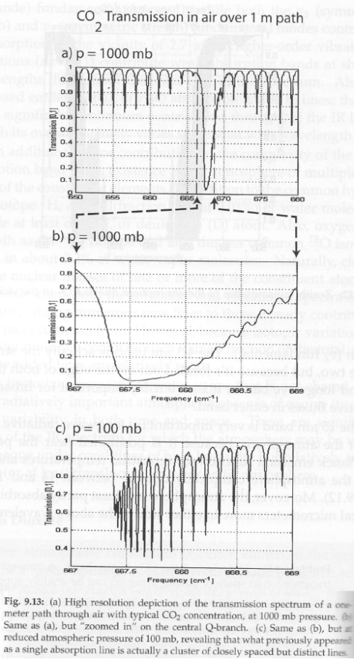
Here’s the value through a 1m path around the better known peak absorption of CO2 at wavenumbers around 667cm-1 = wavelengths around 15μm:

From Grant Petty (2006)

Fascinating stuff. As you can see 95% of radiation at 15μm is absorbed in just 1 meter of atmosphere at the surface of the earth (1000 mb).

Amazing, considering that CO2 is only 370ppm or thereabouts.

You can see the effect of what is called “pressure broadening” of the individual lines with the 1000mb (surface pressure) vs the 100mb (about 16km altitude) value.

This is something we will return to in a later article.

Many people write about the strong absorption of CO2 at 667 cm-1 / 15μm without commenting on the absorption at 600 cm-1 or 750 cm-1.

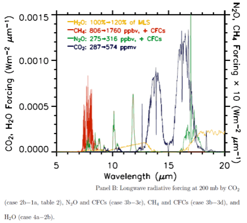
The less strong absorption around the “wings” of the band is the reason for this graph below of the wavelength dependent impact of a doubling of CO2 (from pre-industrial levels) on the “radiative forcing”:

Longwave radiative forcing from increases in various "greenhouse" gases

Longwave radiative forcing from increases in various "greenhouse" gases

From Radiative forcing by well-mixed greenhouse gases: Estimates from climate models in the IPCC AR4, W.D. Collins et al, Journal of Geophysical Research (2006). Note that the vertical axis units are incorrect.

Early comments on CO2 in the HITRAN database

There are almost 315,000 individual absorption lines for CO2 recorded in the database. The database has 2.7M absorption lines in total for 39 molecules.

Between 665 – 669 cm-1 there are over 2,000 lines.

Between 647 – 687 cm-1 there are over 16,000 lines.

Between 500 – 800 cm-1 (12.5 μm – 20μm) there are almost 63,000 lines.

Over 248,000 lines for CO2 are above 800 cm-1 , i.e., between 0-12.5 μm.

The main reference paper for HITRAN 2008 (see below) says:

The present atmospheric version of CDSD (Carbon Dioxide Spectroscopic Databank) consists of 419,610 lines .. covering a wavenumber range of 5–12784 cm-1.

– so I’m not sure whether not all of them made it into the HITRAN database, or whether I have missed something important.

Now that I’ve read the database into some Matlab arrays I will have a tinker around and see if I can come up with the same kind of calculations as people like Grant Petty.

If I can’t, I will immediately announce that climate science has made a huge mistake, write up my results and become the next internet-celebrated debunker of atmospheric physics.

Or, I’ll try and figure out why I got a different result from all the people who know so much more than me..

Other articles in the series:

Part One – a bit of a re-introduction to the subject.

Part Two – introducing a simple model, with molecules pH2O and pCO2 to demonstrate some basic effects in the atmosphere. This part – absorption only.

Part Three – the simple model extended to emission and absorption, showing what a difference an emitting atmosphere makes. Also very easy to see that the “IPCC logarithmic graph” is not at odds with the Beer-Lambert law.

Part Four – the effect of changing lapse rates (atmospheric temperature profile) and of overlapping the pH2O and pCO2 bands. Why surface radiation is not a mirror image of top of atmosphere radiation.

Part Five – a bit of a wrap up so far as well as an explanation of how the stratospheric temperature profile can affect “saturation”

Part Six – The Equations – the equations of radiative transfer including the plane parallel assumption and it’s nothing to do with blackbodies

Part Seven – changing the shape of the pCO2 band to see how it affects “saturation” – the wings of the band pick up the slack, in a manner of speaking

Part Eight – interesting actual absorption values of CO2 in the atmosphere from Grant Petty’s book

Part Nine – calculations of CO2 transmittance vs wavelength in the atmosphere using the 300,000 absorption lines from the HITRAN database

Part Ten – spectral measurements of radiation from the surface looking up, and from 20km up looking down, in a variety of locations, along with explanations of the characteristics

Part Eleven – Heating Rates – the heating and cooling effect of different “greenhouse” gases at different heights in the atmosphere

Part Twelve – The Curve of Growth – how absorptance increases as path length (or mass of molecules in the path) increases, and how much effect is from the “far wings” of the individual CO2 lines compared with the weaker CO2 lines

And Also –

Theory and Experiment – Atmospheric Radiation – real values of total flux and spectra compared with the theory.

References

The reference describing the HITRAN database:

The HITRAN 2008 molecular spectroscopic database, L.S. Rothman et al, Journal of Quantitative Spectroscopy & Radiative Transfer 110 (2009) 533–572

Read Full Post »