Feeds:
Posts
Comments

Archive for May, 2017

I probably should have started a separate series on rainfall and then woven the results back into the Impacts series. It might take a few articles working through the underlying physics and how models and observations of current and past climate compare before being able to consider impacts.

There are a number of different ways to look at rainfall models and reality:

  • What underlying physics provides definite constraints regardless of individual models, groups of models or parameterizations?
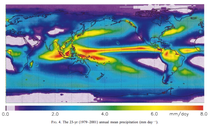
  • How well do models represent the geographical distribution of rain over a climatological period like 30 years? (e.g. figure 8 in Impacts XI – Rainfall 1)
  • How well do models represent the time series changes of rainfall?
  • How well do models represent the land vs ocean? (when we think about impacts, rainfall over land is what we care about)
  • How well do models represent the distribution of rainfall and the changing distribution of rainfall, from lightest to heaviest?

In this article I thought I would highlight a set of conclusions from one paper among many. It’s a good starting point. The paper is A canonical response of precipitation characteristics to global warming from CMIP5 models by Lau and his colleagues, and is freely available, and as always I recommend people read the whole paper, along with the supporting information that is also available via the link.

As an introduction, the underlying physics perhaps provides some constraints. This is strongly believed in the modeling community. The constraint is a simple one – if we warm the ocean by 1K (= 1ºC) then the amount of water vapor above the ocean surface increases by about 7%. So we expect a warmer world to have more water vapor – at least in the boundary layer (typically 1km) and over the ocean. If we have more water vapor then we expect more rainfall. But GCMs and also simple models suggest a lower value, like 2-3% per K, not 7%/K. We will come back to why in another article.

It also seems from models that with global warming, rainfall increases more in regions and times of already high rainfall and reduces in regions and times of low rainfall – the “wet get wetter and the dry get drier”. (Also a marketing mantra that introducing a catchy slogan ensures better progress of an idea). So we also expect changes in the distribution of rainfall. One reason for this is a change in the tropical circulation. All to be covered later, so onto the paper..

We analyze the outputs of 14 CMIP5 models based on a 140 year experiment with a prescribed 1% per year increase in CO2 emission. This rate of CO2 increase is comparable to that prescribed for the RCP8.5, a relatively conservative business-as-usual scenario, except the latter includes also changes in other GHG and aerosols, besides CO2.

A 27-year period at the beginning of the integration is used as the control to compute rainfall and temperature statistics, and to compare with climatology (1979–2005) of rainfall data from the Global Precipitation Climatology Project (GPCP). Two similar 27-year periods in the experiment that correspond approximately to a doubling of CO2 emissions (DCO2) and a tripling of CO2 emissions (TCO2) compared to the control are chosen respectively to compute the same statistics..

Just a note that I disagree with the claim that RCP8.5 is a “relatively conservative business as usual scenario” (see Impacts – II – GHG Emissions Projections: SRES and RCP), but that’s just an opinion, as are all views about where the world will be in population, GDP and cumulative emissions 100-150 years from now. It doesn’t detract from the rainfall analysis in the paper.

For people wondering “what is CMIP5?” – this is the model inter-comparison project for the most recent IPCC report (AR5) where many models have to address the same questions so they can be compared.

Here we see (and along with other graphs you can click to enlarge) what the models show in temperature (top left), mean global rainfall (top right), zonal rainfall anomaly by latitude (bottom left) and the control vs the tripled CO2 comparison (bottom right). The many different colors in the first three graphs are each model, while the black line is the mean of the models (“ensemble mean”). The bottom right graph helps put the changes shown in the bottom left into a perspective – with the different between the red and the blue being the difference between tripling CO2 and today:
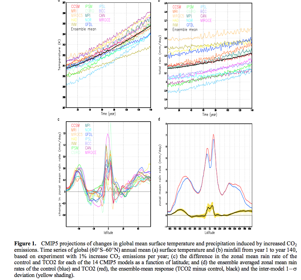
From Lau et al 2013

Figure 1 – Click to enlarge

In the figure above, the bottom left graph shows anomalies. We see one of the characteristics of models as a result of more GHGs – wetter tropics and drier sub-tropics, along with wetter conditions at higher latitudes.

From the supplementary material, below we see a better regional breakdown of fig 1d (bottom right in the figure above). I’ll highlight the bottom left graph (c) for the African region. Over the continent, the differences between present day and tripling CO2 seem minor as far as model predictions go for mean rainfall:
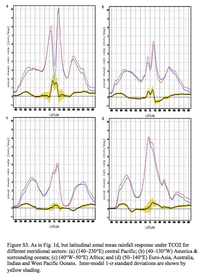
From Lau et al 2013

Figure 2 – Click to enlarge

The supplementary material also has a comparison between models and observations. The first graph below is what we are looking at (the second graph we will consider afterwards). TRMM (Tropical Rainfall Measuring Mission) is satellite data and GPCP one rainfall climatology that we met in the last article – so they are both observational datasets. We see that the models over-estimate tropic rainfall, especially south of the equator:
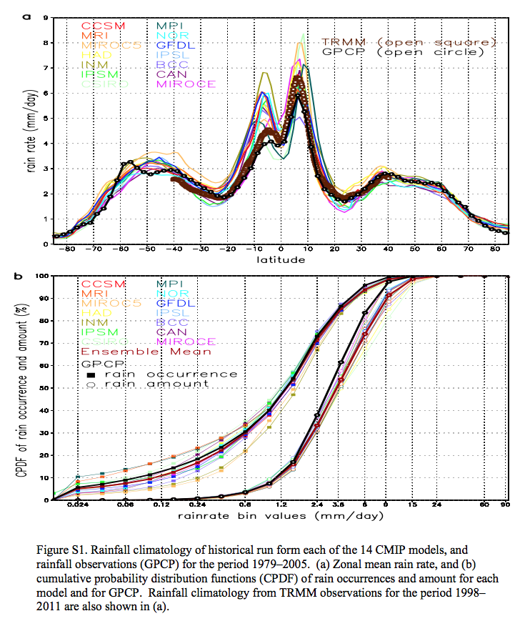
From Lau et al 2013

Figure 3 – Click to enlarge

Rainfall Distribution from Light through to Heavy Rain

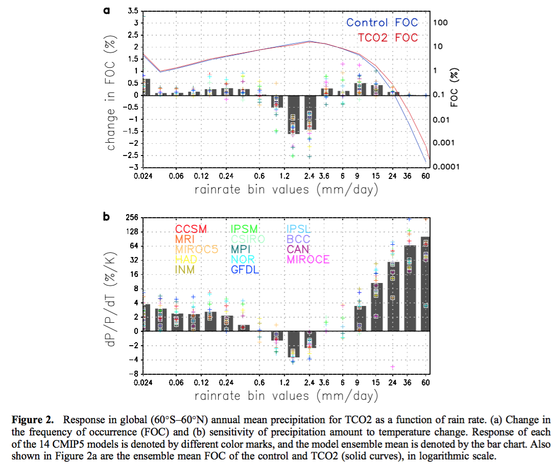
Lau and his colleagues then look at rainfall distribution in terms of light rainfall through to heavier rainfall. So, take global rainfall and divide it into frequency of occurrence, with light rainfall to the left and heavy rainfall to the right. Take a look back at the bottom graph in the figure above (figure 3, their figure S1). Note that the horizontal axis is logarithmic, with a ratio of over 1000 from left to right.

It isn’t an immediately intuitive graph. Basically there are two sets of graphs. The left “cluster” is how often that rainfall amount occurred, and the black line is GPCP observations. The “right cluster” is how much rainfall fell (as a percentage of total rainfall) for that rainfall amount and again black is observations.

So lighter rainfall, like 1mm/day and below accounts for 50% of time, but being light rainfall accounts for less than 10% of total rainfall.

To facilitate discussion regarding rainfall characteristics in this work, we define, based on the ensemble model PDF, three major rain types: light rain (LR), moderate rain (MR), and heavy rain (HR) respectively as those with monthly mean rain rate below the 20th percentile (<0.3 mm/day), between response (TCO2 minus control, black) and the inter-model 1s the 40th–70th percentile (0.9–2.4mm/day), and above the 98.5% percentile (>9mm/day). An extremely heavy rain (EHR) type defined at the 99.9th percentile (>24 mm day1) will also be referred to, as appropriate.

Here is a geographical breakdown of the total and then the rainfall in these three categories, model mean on the left and observations on the right:
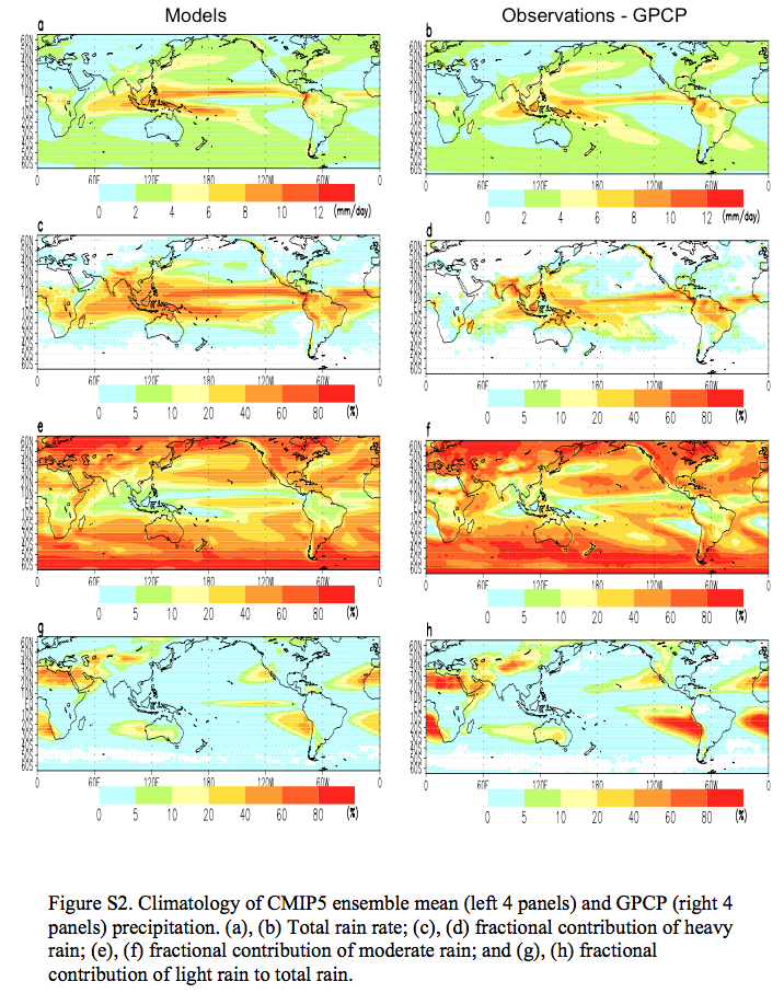
From Lau et al 2013

Figure 4 – Click to enlarge

We can see that the models tend to overestimate the heavy rain and underestimate the light rain. These graphics are excellent because they help us to see the geographical distribution.

Now in the graphs below we see at the top the changes in frequency of mean precipitation (60S-60N) as a function of rain rate; and at the bottom we see the % change in rainfall per K of temperature change, again as a function of rain rate. Note that the bottom graph also has a logarithmic scale for the % change, so as you move up each grid square the value is doubled.

The different models are also helpfully indicated so the spread can be seen:

From Lau et al 2013

Figure 5 – Click to enlarge

Notice that the models are all predicting quite a high % change in rainfall per K for the heaviest rain – something around 50%. In contrast the light rainfall is expected to be up a few % per K and the medium rainfall is expected to be down a few % per K.

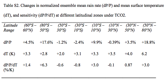
Globally, rainfall increases by 4.5%, with a sensitivity (dP/P/dT) of 1.4% per K

Here is a table from their supplementary material with a zonal breakdown of changes in mean rainfall (so not divided into heavy, light etc). For the non-maths people the first row, dP/P is just the % change in precipitation (“d” in front of a variable means “change in that variable”), the second row is change in temperature and the third row is the % change in rainfall per K (or ºC) of warming from GHGs:

From Lau et al 2013

Figure 6 – Click to enlarge

Here are the projected geographical distributions of the changes in mean (top left), heavy (top right), medium (bottom left) and light rain (bottom right) – using their earlier definitions – under tripling CO2:
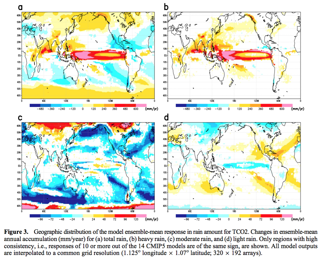
From Lau et al 2013

Figure 7 – Click to enlarge

And as a result of these projections, the authors also show the number of dry months and the projected changes in number of dry months:
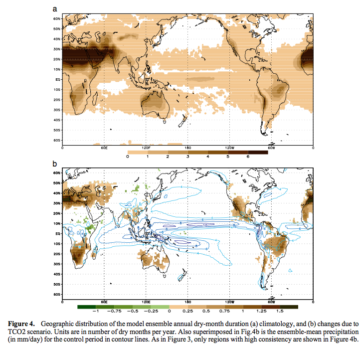
From Lau et al 2013

Figure 8 – Click to enlarge

The authors conclude:

The IPCC CMIP5 models project a robust, canonical global response of rainfall characteristics to CO2 warming, featuring an increase in heavy rain, a reduction in moderate rain, and an increase in light rain occurrence and amount globally.

For a scenario of 1% CO2 increase per year, the model ensemble mean projects at the time of approximately tripling of the CO2 emissions, the probability of occurring of extremely heavy rain (monthly mean >24mm/day) will increase globally by 100%–250%, moderate rain will decrease by 5%–10% and light rain will increase by 10%–15%.

The increase in heavy rain is most pronounced in the equatorial central Pacific and the Asian monsoon regions. Moderate rain is reduced over extensive oceanic regions in the subtropics and extratropics, but increased over the extratropical land regions of North America, and Eurasia, and extratropical Southern Oceans. Light rain is mostly found to be inversely related to moderate rain locally, and with heavy rain in the central Pacific.

The model ensemble also projects a significant global increase up to 16% more frequent in the occurrences of dry months (drought conditions), mostly over the subtropics as well as marginal convective zone in equatorial land regions, reflecting an expansion of the desert and arid zones..


..Hence, the canonical global rainfall response to CO2 warming captured in the CMIP5 model projection suggests a global scale readjustment involving changes in circulation and rainfall characteristics, including possible teleconnection of extremely heavy rain and droughts separated by far distances. This adjustment is strongly constrained geographically by climatological rainfall pattern, and most likely by the GHG warming induced sea surface temperature anomalies with unstable moister and warmer regions in the deep tropics getting more heavy rain, at the expense of nearby marginal convective zones in the tropics and stable dry zones in the subtropics.

Our results are generally consistent with so-called “the rich-getting-richer, poor-getting-poorer” paradigm for precipitation response under global warming..

Conclusion

This article has basically presented the results of one paper, which demonstrates consistency in model response of rainfall to doubling and tripling of CO2 in the atmosphere. In subsequent articles we will look at the underlying physics constraints, at time-series over recent decades and try to make some kind of assessment.

Articles in this Series

Impacts – I – Introduction

Impacts – II – GHG Emissions Projections: SRES and RCP

Impacts – III – Population in 2100

Impacts – IV – Temperature Projections and Probabilities

Impacts – V – Climate change is already causing worsening storms, floods and droughts

Impacts – VI – Sea Level Rise 1

Impacts – VII – Sea Level 2 – Uncertainty

Impacts – VIII – Sea level 3 – USA

Impacts – IX – Sea Level 4 – Sinking Megacities

Impacts – X – Sea Level Rise 5 – Bangladesh

Impacts XI – Rainfall 1

References

A canonical response of precipitation characteristics to global warming from CMIP5 models, William K.-M. Lau, H.-T. Wu, & K.-M. Kim, GRL (2013) – free paper

Further Reading

Here are a bunch of papers that I found useful for readers who want to dig into the subject. Most of them are available for free via Google Scholar, but one of the most helpful to me (first in the list) was Allen & Ingram 2002 and the only way I could access it was to pay $4 to rent it for a couple of days.

Allen MR, Ingram WJ (2002) Constraints on future changes in climate and the hydrologic cycle. Nature 419:224–232

Allan RP (2006) Variability in clear-sky longwave radiative cooling of the atmosphere. J Geophys Res 111:D22, 105

Allan, R. P., B. J. Soden, V. O. John, W. Ingram, and P. Good (2010), Current changes in tropical precipitation, Environ. Res. Lett., doi:10.1088/ 1748-9326/5/52/025205

Physically Consistent Responses of the Global Atmospheric Hydrological Cycle in Models and Observations, Richard P. Allan et al, Surv Geophys (2014)

Held IM, Soden BJ (2006) Robust responses of the hydrological cycle to global warming. J Clim 19:5686–5699

Changes in temperature and precipitation extremes in the CMIP5 ensemble, VV Kharin et al, Climatic Change (2013)

Energetic Constraints on Precipitation Under Climate Change, Paul A. O’Gorman et al, Surv Geophys (2012) 33:585–608

Trenberth, K. E. (2011), Changes in precipitation with climate change, Clim. Res., 47, 123–138, doi:10.3354/cr00953

Zahn M, Allan RP (2011) Changes in water vapor transports of the ascending branch of the tropical circulation. J Geophys Res 116:D18111

Read Full Post »

If we want to assess forecasts of floods, droughts and crop yields then we will need to know rainfall. We will also need to know temperature of course.

The forte of climate models is temperature. Rainfall is more problematic.

Before we get to model predictions about the future we need to review observations and the ability of models to reproduce them. Observations are also problematic – rainfall varies locally and over short durations. And historically we lacked effective observation systems in many locations and regions of the world, so data has to be pieced together and estimated from reanalysis.

Smith and his colleagues created a new rainfall dataset. Here is a comment from their 2012 paper:

Although many land regions have long precipitation records from gauges, there are spatial gaps in the sampling for undeveloped regions, areas with low populations, and over oceans. Since 1979 satellite data have been used to fill in those sampling gaps. Over longer periods gaps can only be filled using reconstructions or reanalyses..

Here are two views of the global precipitation data from a dataset which starts with the satellite era, that is, 1979 onwards – GPCP (Global Precipitation Climatology Project):

From Adler et al 2003

Figure 1

From Adler et al 2003

Figure 2

For historical data before satellites we only have rain gauge data. The GPCC dataset, explained in Becker et al 2013, shows the number of stations over time by region:

From Becker et al 2013

Figure 3- Click to expand

And the geographical distribution of rain gauge stations at different times:

From Becker et al 2013

Figure 4 – Click to expand

The IPCC compared the global trends over land from four different datasets over the last century and the last half-century:

From IPCC AR5 Ch. 2

Figure 5 – Click to expand

And the regional trends:

From IPCC AR5 Ch. 2

Figure 6 – Click to expand

The graphs for the annual change in rainfall, note the different scales for each region (as we would expect given the difference in average rainfall in different region):

From IPCC AR5 ch 2

Figure 7

We see that the decadal or half-decadal variation is much greater than any apparent long term trend. The trend data (as reviewed by the IPCC in figs 5 & 6) shows significant differences in the datasets but when we compare the time series it appears that the datasets match up better than indicated by the trend comparisons.

The data with the best historical coverage is 30ºN – 60ºN and the trend values for 1951-2000 (from different reconstructions) range from an annual increase of 1 to 1.5 mm/yr per decade (fig 6 / table 2.10 of IPCC report). This is against an absolute value of about 1000 mm/yr in this region (reading off the climatology in figure 2).

This is just me trying to put the trend data in perspective.

Models

Here is the IPCC AR5 chapter 9 on model comparisons to satellite-era rainfall observations. Top left is observations (basically the same dataset as figure 1 in this article over a slightly longer period with different colors) and bottom right is percentage error of model average with respect to observations:

From IPCC AR5 ch 9

Figure 8 – Click to expand

We can see that the average of all models has substantial errors on mean rainfall.

Articles in this Series

Impacts – I – Introduction

Impacts – II – GHG Emissions Projections: SRES and RCP

Impacts – III – Population in 2100

Impacts – IV – Temperature Projections and Probabilities

Impacts – V – Climate change is already causing worsening storms, floods and droughts

Impacts – VI – Sea Level Rise 1

Impacts – VII – Sea Level 2 – Uncertainty

Impacts – VIII – Sea level 3 – USA

Impacts – IX – Sea Level 4 – Sinking Megacities

Impacts – X – Sea Level Rise 5 – Bangladesh

References

IPCC AR5 Chapter 2

Improved Reconstruction of Global Precipitation since 1900, Smith, Arken, Ren & Shen, Journal of Atmospheric and Oceanic Technology (2012)

The Version-2 Global Precipitation Climatology Project (GPCP) Monthly Precipitation Analysis (1979–Present), Adler et al, Journal of Hydrometeorology (2003)

A description of the global land-surface precipitation data products of the Global Precipitation Climatology Centre with sample applications including centennial (trend) analysis from 1901–present, A Becker, Earth Syst. Sci. Data (2013)

Read Full Post »

FitzGerald et al 2008:

Sea-level rise (SLR) poses a particularly ominous threat because 10% of the world’s population (634 million people) lives in low-lying coastal regions within 10 m elevation of sea level (McGranahan et al. 2007). Much of this population resides in portions of 17 of the world’s 30 largest cities, including Mumbai, India; Shanghai, China; Jakarta, Indonesia; Bangkok, Thailand; London; and New York.

In the last article – Sinking Megacities – we saw that some of these cities are sinking due to ground water depletion. To those megacities, this is a much more serious threat than global sea level rise (probably why we see so many marches and protests about ground water depletion).

The paper continues:

..The potential loss of life in low-lying areas is even more graphically illustrated by the 1970 Bhola cyclone that traveled northward through the Bay of Bengal producing a 12-m-high wall of water that drowned a half million people in East Pakistan (now Bangladesh) (Garrison 2005).

In Bangladesh, storms and cyclones are much more of a threat than sea level rise. Here is Karim and Mimura (2008) listing the serious cyclones over the last 60 years:

From Karim and Mimura 2008

Figure 1 – Click to expand

There is an interesting World Bank Report from 2011. First on floods:

In an average year, nearly one quarter of Bangladesh is inundated, with more than three-fifths of land area at risk of floods of varying intensity (Ahmed and Mirza 2000). Every four or five years, a severe flood occurs during the monsoon season, submerging more than three-fifths of the land..

The most recent exceptional flood, which occurred in 2007, inundated 62,300 km² or 42 percent of total land area, causing 1,110 deaths and affecting 14 million people; 2.1 million ha of standing crop land were submerged, 85,000 houses completely destroyed, and 31,533 km of roads damaged. Estimated asset losses from this one event totaled US$1.1 billion (BWDB 2007).

Flooding in Bangladesh results from a complex set of factors, key among which are extremely low and flat topography, uncertain transboundary flow, heavy monsoon rainfall, and high vulnerability to tidal waves and congested drainage channels. Two-thirds of Bangladesh’s land area is less than 5 m above sea level. Each year, an average flow of 1,350 billion m³ of water from the GBM [Ganges, Brahmaputra, and Meghna] basin drains through the country.

From World Bank 2011

Figure 2

I recommend this World Bank report, very interesting, and you can see some idea of the costs of mitigating against floods. These problems are already present – floods are a regular occurrence, some mitigation has already taken place, and more mitigation continues.

I read the entire report and all I could find was that rising sea levels would exacerbate the problems already faced from storm surges: p.6:

Increase in ocean surface temperature and rising sea levels are likely to intensify cyclonic storm surges and further increase the depth and extent of storm surge induced coastal inundation.

However, the projections indicate that sea level rise is much less of a problem compared with possible increases in future storm surges and possible increases in future flooding. And compared with current storm surges and current flooding. We will look at floods and storm surges in future articles.

In the report it’s clear that floods and storms are already major problems. Sea level is harder to analyze. Trying to account for a sea level rise of 0.3m by 2050 when severe storm surges are already 5-10m is not going to make much of a difference. If we had accurate prediction of storm surges, to +/- 0.3m, then sea level rise of 0.3m should definitely be accounted for. But we don’t have anything like that kind of accuracy.

Well, they do some calculations of adaption against storm surges for projected changes up to 2050:

Under the baseline scenario, the adaptation costs total $2.46 billion. In a changing climate, the additional adaptation cost totals US$892 million.

In essence the question is “what is the storm surge for a once in a 10 year storm in 2050”? (I’m sure Bangladesh would really prefer to build protection against a once in 100 year storm). An extra $1bn for future problems, or a total of $3.5bn to cover existing and future problems, seems like money that would be very well spent, representing excellent value.

Nicholls and Cazenave (2010), in relation to the susceptible coastline of Asia and Africa, comment on adaption:

Many impact studies do not consider adaptation, and hence determine worst-case impacts. Yet, the history of the human relationship with the coast is one of an increasing capacity to adapt to adverse change. In addition, the world’s populated coasts became increasingly managed and engineered over the 20th century. The subsiding cities discussed above all remain protected to date, despite large relative SLR.

Analysis based on benefit-cost methods show that protection would be widespread as well-populated coastal areas have a high value and actual impacts would only be a small fraction of the potential impacts, even assuming high-SLR (>1 m/century) scenarios. This suggests that the common assumption of a widespread forced retreat from the shore in the face of SLR is not inevitable. In many densely populated coastal areas, communities advanced the coast seaward via land claim owing to the high value of land (e.g., Singapore).

Yet, protection often attracts new development in low lying areas, which may not be desirable, and coastal defense failures have occurred, such as New Orleans in 2005. Hence, we must choose between protection, accommodation, and planned retreat adaptation options. This choice is both technical and sociopolitical, addressing which measures are desirable, affordable, and sustainable in the long term. Adaptation remains a major uncertainty concerning the actual impacts of SLR.

In the World Bank 2011 report, in chapter 4, after their analysis on risks and costs of storm-induced inundations in 2050 resulting from projected higher cyclonic wind speeds and a projected increase in sea level of 0.27m, they comment, p.24:

As a cautionary note, it should be noted that this analysis did not address the out-migration from coastal zones that a rise in sea level and intensified cyclonic storm surges might induce.

In fact the cost data assumes population growth in the vulnerable regions.

Likewise, here is Hinkel et al (2014):

Coastal flood damages are expected to increase significantly during the 21st century as sea levels rise and socioeconomic development increases the number of people and value of assets in the coastal floodplain.

[Emphasis added].

This assumption bias creates an interpretation challenge. It would be useful to see notes to the effect: “If the population migrates away from this area due to the higher risk, instead the cost will be $X assuming a reduction of Y% in population in this region by 2050“. This extra item of data would create a useful contrast and I’m guessing that we would see impact assessments reduce by a factor of 5 or 10.

It is difficult to see realistic global sea level changes, even to the end of the century, having a big impact on Bangladesh compared with their current problems of annual flooding and frequent large storm surges. Of course, adding an extra 0.5m to the sea level doesn’t improve the situation, but it is an order of magnitude smaller than storm surges.

The adaption costs estimated by the World Bank to protect against storm surges (already required but at least a work in progress) seem moderate in value.

Lastly, I wasn’t able to find a detailed elevation map (with, say, 0.5m resolution), instead the ones I found graded the elevation with respect to sea level in fairly coarse steps. I’m sure the information exists but may be proprietary (in GIS data for example):

Figure 2 – Click to expand

I have to admit that I believed something like 25% of the Bangladesh population were around 1.0m or less above current sea level. This map says that the 0-3m area is quite small. If anyone does have a better resolution map I will post it up.

Articles in this Series

Impacts – I – Introduction

Impacts – II – GHG Emissions Projections: SRES and RCP

Impacts – III – Population in 2100

Impacts – IV – Temperature Projections and Probabilities

Impacts – V – Climate change is already causing worsening storms, floods and droughts

Impacts – VI – Sea Level Rise 1

Impacts – VII – Sea Level 2 – Uncertainty

Impacts – VIII – Sea level 3 – USA

Impacts – IX – Sea Level 4 – Sinking Megacities

References

Coastal Impacts Due to Sea-Level Rise, Duncan M. FitzGerald et al, Annual Rev. Earth Planet. Sci. (2008)

Impacts of climate change and sea-level rise on cyclonic storm surge floods in Bangladesh, Mohammed Fazlul Karim & Nobuo Mimura, Global Environmental Change (2008) – free paper

The Cost of Adapting to Extreme Weather Events in a Changing Climate – Bangladesh, World Bank (2011) – free report

Sea-Level Rise and Its Impact on Coastal Zones, Robert J Nicholls & Anny Cazenave, Science (2010) – free paper

Coastal flood damage and adaptation costs under 21st century sea-level rise, Jochen Hinkel et al, PNAS (2014) – free paper

Read Full Post »

In Impacts – VIII – Sea level 3 – USA I suggested this conclusion:

So the cost of sea level rise for 2100 in the US seems to be a close to zero cost problem.

Probably the provocative way I wrote the conclusion confused some people. I should have said that it was a very expensive problem. But that it wasn’t a problem that society should pay for, given that anyone moving to the coast since 2005 at the latest would have known that future sea level was considered to be a major problem. By 2100 the youngest people still living right on the sea front, who bought property there before 2005, would be at least 115 years old.

The idea is that “externalities” as economists call them should be paid by the creators of the problem, not the people that incur the problem. In this case, the “victims” are people who ignored the evidence and moved to the coast anyway. Are they still victims? That was my point.

Well, what about outside the US?

Some mega cities have huge problems. Here is Nicholls 2011:

Coastal areas constitute important habitats, and they contain a large and growing population, much of it located in economic centers such as London, New York, Tokyo, Shanghai, Mumbai, and Lagos. The range of coastal hazards includes climate-induced sea level rise, a long-term threat that demands broad response.

Global sea levels rose 17 cm through the twentieth century, and are likely to rise more rapidly through the twenty-first century when a rise of more than 1 m is possible.

In some locations, these changes may be exacerbated by

(1) increases in storminess due to climate change, although this scenario is less certain
(2) widespread human-induced subsidence due to ground fluid withdrawal from, and drainage of, susceptible soils, especially in deltas.

Subsidence?

Over the twentieth century, the parts of Tokyo and Osaka built on deltaic areas subsided up to 5 m and 3 m, respectively, a large part of Shanghai subsided up to 3 m, and Bangkok subsided up to 2 m.

This human-induced subsidence can be mitigated by stopping shallow, subsurface fluid withdrawals and managing water levels, but natural “background” rates of subsidence will continue, and RSLR will still exceed global trends in these areas. A combination of policies to mitigate subsidence has been instituted in the four delta cities mentioned above, combined with improved flood defenses and pumped drainage systems designed to avoid submergence and/ or frequent flooding.

In contrast, Jakarta and Metro Manila are subsiding significantly, with maximum subsidence of 4 m and 1 m to date, respectively (e.g., Rodolfo and Siringan, 2006; Ward et al., 2011), but little systematic policy response is in place in either city, and future flooding problems are anticipated.

Subsidence graphic:

From Nicholls 2011

Figure 1

To put these figures in context, sea level rise from 1900-2000 was about 0.2m and according to the latest IPCC report the forecast of sea level rise by 2100 might be around an additional 0.5m (for RCP 6.0, see earlier article). In the light of the idea that global society should pay for problems to people caused by global society, perhaps the problems of Shanghai, Bangkok and other sinking cities are not global problems?

Here is Wang et al from 2012:

Shanghai is low-lying, with an elevation of 3–4 m. A quarter of the area lies below 3 m. The city’s flood-control walls are currently more than 6 m high. However, given the trend of sea level rise and land subsidence, this is inadequate. Shanghai is frequently affected by extreme tropical storm surges. The risk of flooding from overtopping is considerable..

..From 1921 to 1965, the average cumulative subsidence of the city center was 1.76 m, with a maximum of 2.63 m. From 1966 to 1985, a monitoring network was established and subsidence was mitigated through artificial recharge. Land subsidence was stabilized at an average of 0.9 mm/year. As a result of rapid urban development and large-scale construction projects between 1986 and 1997, subsidence of the downtown area increased rapidly, at an average rate of 10.2 mm/year..

..In 2100, sea level rise and land subsidence will be far greater than before. Sea level rise is estimated to be 43 cm, while land subsidence is estimated to be 3–229 cm, and neotectonic subsidence is estimated to be 14 cm. Flooding will be severe in 2100 (Fig. 8).

[Note I changed the data in the last paragraph cited to round numbers in cm from their values quoted to 0.01cm – for example, 43cm instead of the paper’s values of 43.31 etc].

So for Shanghai at least global sea level rise is not really the problem.

Given that I don’t pay much attention to media outlets I probably missed the big Marches against Ground Water Depletion Slightly Accentuating Global Warming’s Sea Level Rise in Threatened Megacities.

As with the USA data the question of increased storm surges accentuating global sea level rise is still on the agenda (i.e., has not yet been discussed).

References

Planning for the impacts of sea level rise, RJ Nicholls, Oceanography (2011)

Evaluation of the combined risk of sea level rise, land subsidence, and storm surges on the coastal areas of Shanghai, China, Jun Wang, Wei Gao, Shiyuan Xu & Lizhong Yu, Climatic Change (2012)


Read Full Post »