In previous articles in this series we looked at a number of issues first in Miskolczi’s 2010 paper and then in the 2007 paper.
The author himself has shown up and commented on some of these points, although not all, and sadly decided that we are not too bright and a little bit too critical and better pastures await him elsewhere.
Encouraged by one of our commenters I pressed on into the paper: Greenhouse Effect in Semi-Transparent Planetary Atmospheres, Quarterly Journal of the Hungarian Meteorological Service (2007), and now everything is a lot clearer.
The 2007 paper by Ferenc Miskolczi is a soufflé of confusion piled on confusion. Sorry to be blunt. If I was writing a paper I would say “..some clarity is needed in important sections..” but many readers unfamiliar with the actual meaning of this phrase might think that some clarity was needed in important sections rather than the real truth that the paper is a shambles.
I’ll refer to this paper as M2007. And to the equations in M2007 with an M prefix – so, for example, equation 15 will be [M15].
Some background is needed so first we need to take a look at something called The Semi-Gray Model. Regular readers will find a lot of this to be familiar ground, but it is necessary as there are always many new readers.
The SGM – Semi-Grey Model or Schwarzschild Grey Model
I’ll introduce this by quoting from an excellent paper referenced by M2007. This is a 1995 paper by Weaver and the great Ramanathan (free link in References):
Simple models of complex systems have great heuristic value, in that their results illustrate fundamental principles without being obscured by details. In particular, there exists a long history of simple climate models. Of these, radiative and radiative-convective equilibrium models have received great attention..
One of the simplest radiative equilibrium models involves the assumption of a so-called grey atmosphere, where the absorption coefficient is assumed to be independent of wavelength. This was first discussed by Schwarzschild [1906] in the context of stellar interiors. The grey gas model was adapted to studies of the Earth by assuming the atmosphere to be transparent to solar radiation and grey for thermal radiation. We will refer to this latter class as semigrey models.
And in the abstract they say:
Radiative equilibrium solutions are the starting point in our attempt to understand how the atmospheric composition governs the surface and atmospheric temperatures, and the greenhouse effect. The Schwarzschild analytical grey gas model (SGM) was the workhorse of such attempts. However, the solution suffered from serious deficiencies when applied to Earth’s atmosphere and were abandoned about 3 decades ago in favor of more sophisticated computer models..
[Emphasis added]
And they go on to present a slightly improved SGM as a useful illustrative tool.
Some clarity on a bit of terminology for new readers – a blackbody is a perfect emitter and absorber of radiation. In practice there are no blackbodies but some bodies come very close. A blackbody has an emissivity = 1 and absorptivity = 1.
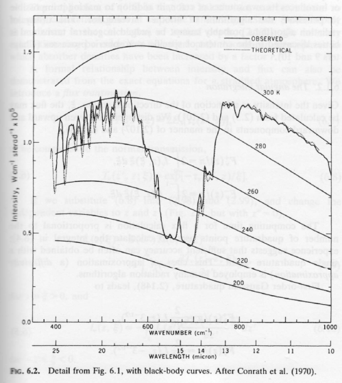
In our atmosphere, the gases which absorb and emit significant radiation have very wavelength dependent properties, e.g.:

From spectralcalc.com
Figure 1
So the emissivity and absorptivity vary hugely from one wavelength to the next (note 1). However, as an educational tool, we can calculate the results for a grey atmosphere – this means that the emissivity is assumed to be constant across all wavelengths.
The term semi-grey means that the atmosphere is considered transparent for shortwave = solar wavelengths (<4 μm) and constant but not zero for longwave = terrestrial wavelengths (>4 μm).
Constructing the SGM
This model is very simple – and is not used to really calculate anything of significance for our climate. See Understanding Atmospheric Radiation and the “Greenhouse” Effect – Part Six – The Equations for the real equations.
We assume that the atmosphere is in radiative equilibrium – that is, convection does not exist and so only radiation moves heat around.
Here is a graphic showing the main elements of the model:

Figure 2
Once each layer in the atmosphere is in equilibrium, there is no heating or cooling – this is the definition of equilibrium. This means energy into the layer = energy out of the layer. So we can use simple calculus to write some equations of radiative transfer.
We define the TOA (top of atmosphere) to be where optical thickness, τ=0, and it increases through the atmosphere to reach a maximum of τ=τA at the surface. This is conventional.
We also know two boundary conditions, because at TOA (top of atmosphere) the downward longwave flux, F↓(τ=0) = 0 and the upwards longwave flux, F↑(τ=0) = F0, where F0 = absorbed solar radiation ≈ 240 W/m². This is because energy leaving the planet must be balanced by energy being absorbed by the planet from the sun.
We also have to consider the fact that energy is not just going directly up and down but is going up and down at every angle. We can deal with this via the dffusivity approximation which sums up the contributions from every angle and tells us that if we use τ*= τ . 5/3 (where τ is defined in the vertical direction) we get the complete contribution from all of the different directions. (Note 2). For those following M2007 I have used τ* to be his τ with a ˜ on top, and τ to be his τ with a ¯ on top.
With these conditions we can get a solution for the SGM (see derivation in the comments):
B(τ) = F0/2π . (τ+1) [1] cf eqn [M15]
where B is the spectrally integrated Planck function, and remember F0 is a constant.
And also:
F↑(τ) = F0/2 . (τ+2) [2]
F↓(τ) = F0/2 . τ [3]
A quick graphic might explain this a little more (with an arbitrary total optical thickness, τA* = 3):

Figure 3
Notice that the upward longwave flux at TOA is 240 W/m² – this balances the absorbed solar radiation. And the downward longwave flux at TOA is zero, because there is no atmosphere above from which to radiate. This graph also demonstrates that the difference between F↑ and F↓ is a constant as we move through the atmosphere, meaning that the heating rate is zero. The increase in downward flux, F↓, is matched by the decrease in upward flux, F↑.
It’s a very simple model.
By contrast, here are the heating/cooling rates from a comprehensive (= “standard”) radiative-convective model, plotted against height instead of optical thickness.
Heating from solar radiation, because the atmosphere is not completely transparent to solar radiation:

From Grant Petty (2006)
Figure 4
Cooling rates due to various “greenhouse” gases:

From Petty (2006)
Figure 5
And the heating and cooling rates won’t match up because convection moves heat from the surface up into the atmosphere.
Note that if we plotted the heating rate vs altitude for the SGM it would be a vertical line on 0.0°C/day.
Let’s take a look at the atmospheric temperature profile implied by the semi-grey model:

Figure 6
Now a lot of readers are probably wondering what the τ really means, or more specifically, what the graph looks like as a function of height in the atmosphere. In this model it very much depends on the concentration of the absorbing gas and its absorption coefficient. Remember it is a fictitious (or “idealized”) atmosphere. But if we assume that the gas is well-mixed (like CO2 for example, but totally unlike water vapor), and the fact that pressure increases with depth then we can produce a graph vs height:

Figure 7
Important note – the values chosen here are not intended to represent our climate system.
Figure 6 & 7, along with figure 3, are just to help readers “see” what a semi-grey model looks like. If we increase the total optical depth of the atmosphere the atmospheric temperature at the surface increases.
Note as well that once the temperature reduction vs height is too large a value, the atmosphere will become unstable to convection. E.g. for a typical adiabatic lapse rate of 6.5 K/km, if the radiative equilibrium implies a lapse rate > 6.5 K/km then convection will move heat to reduce the lapse rate.
Curious Comments on the SGM
Some comments from M2007:
p 11:
Note, that in obtaining B0 , the fact of the semi-infinite integration domain over the optical depth in the formal solution is widely used. For finite or optically thin atmosphere Eq. (15) is not valid. In other words, this equation does not contain the necessary boundary condition parameters for the finite atmosphere problem.
The B0 he is referring to is the constant in [M15]. This constant is H/2π – where H = F0 (absorbed solar radiation) in my earlier notation. This constant B0 later takes on magical properties.
p 12:
Eq. (15) assumes that at the lower boundary the total flux optical depth is infinite. Therefore, in cases, where a significant amount of surface transmitted radiative flux is present in the OLR , Eqs. (16) and (17) are inherently incorrect. In stellar atmospheres, where, within a relatively short distance from the surface of a star the optical depth grows tremendously, this could be a reasonable assumption, and Eq. (15) has great practical value in astrophysical applications. The semi-infinite solution is useful, because there is no need to specify any explicit lower boundary temperature or radiative flux parameter (Eddington, 1916).
[Emphasis added]
The equations can easily be derived without any requirement for the total optical depth being infinite. There is no semi-infinite assumption in the derivation. Whether or not some early derivations included it, I cannot say. But you can find the SGM derivation in many introductions to atmospheric physics and no assumption of infinite optical thickness exists.
When considering the clear-sky greenhouse effect in the Earth’s atmosphere or in optically thin planetary atmospheres, Eq. (16) is physically meaningless, since we know that the OLR is dependent on the surface temperature, which conflicts with the semi-infinite assumption that τA =∞..
..There were several attempts to resolve the above deficiencies by developing simple semi-empirical spectral models, see for example Weaver and Ramanathan (1995), but the fundamental theoretical problem was never resolved..
This is the reason why scientists have problems with a mysterious surface temperature discontinuity and unphysical solutions, as in Lorenz and McKay (2003). To accommodate the finite flux optical depth of the atmosphere and the existence of the transmitted radiative flux from the surface, the proper equations must be derived.
The deficiencies noted include the result in the semi-gray model of a surface air temperature less than the ground temperature. If you read Weaver and Ramanathan (1995) you can see that this isn’t an attempt to solve some “fundamental problem“, but simply an attempt to make a simple model slightly more useful without getting too complex.
The mysterious surface temperature discontinuity exists because the model is not “full bottle”. The model does not include any convection. This discontinuity is not a mystery and is not crying out for a solution. The solution exists. It is called the radiative-convective model and has been around for over 40 years.
Miskolczi makes some further comments on this, which I encourage people to read in the actual paper.
We now move into Appendix B to develop the equations further. The results from the appendix are the equations M20 and M21 on page 14.
Making Equation Soufflé

The highlighted equation is the general solution to the Schwzarschild equation. It is developed in Understanding Atmospheric Radiation and the “Greenhouse” Effect – Part Six – The Equations – the equation reproduced here from that article with explanation:
Iλ(0) = Iλ(τm)e-τm + ∫ Bλ(T)e-τ dτ
The intensity at the top of atmosphere equals..
The surface radiation attenuated by the transmittance of the atmosphere, plus..
The sum of all the contributions of atmospheric radiation – each contribution attenuated by the transmittance from that location to the top of atmosphere
For those wanting to understand the maths a little bit, the 3/2 factor that appears everywhere in Miskolczi’s equation B1 is the diffusivity approximation already mentioned (and see note 2) where we need to sum the radiances over all directions to get flux.
Now this equation is the complete equation of radiative transfer. If we combine it with a simple convective model it is very effective at calculating the flux and spectral intensity through the atmosphere – see Theory and Experiment – Atmospheric Radiation.
So equation B1 in M2007 cannot be solved analytically. This means we have to solve it numerically. This is “simple” in concept but computationally expensive because in the HITRAN database there are 2.7 million individual absorption lines, each one with a different absorption coefficient and a different line width.
However, it can be solved and that is what everyone does. Once you have the database of absorption coefficients and the temperature profile of the atmosphere you can calculate the solution. And band models exist to speed up the process.
And now the rabbit..
The author now takes the equation for the “source function” (B) from the simple model and inserts it into the “complete” solution.
The “source function” in the complete solution can already be calculated – that’s the whole point of the equation B1. But now instead, the source function from the simple model is inserted in its place. This equation assumes that the atmosphere has no convection, has no variation in emissivity with wavelength, has no solar absorption in the atmosphere, and where the heating rate at each level in the atmosphere = zero.

The origin of equation B3 is the equation you see above it:
B(τ) = 3H(τ)/4π + B0 [M13]
Actually, if you check equation M13 on p.11 it is:
B(τ) = 3H.τ/4π + B0 [M13]
This appears to be one of the sources of confusion for Miskolczi, for later comment.
Equation M13 is derived for zero heating rates throughout the atmosphere, and therefore constant H. With this simple assumption – and only for this simple assumption – the equation M13 is a valid solution to “the source function”, ie the atmospheric temperature and radiance.
If you have the complete solution you get one result. If you have the simple model you get a different result. If you take the result from one and stick it in the other how can you expect to get an accurate outcome?
If you want to see how various atmospheric factors are affected by changing τ, then just change τ in the general equation and see what happens. You have to do this via numerical analysis but it can easily be done..
As we continue on working through the appendix, B6 has a sign error in the 2nd term on the right hand side, which is fixed by B7.

This B0 is the constant in the semi-gray solution. The constant appears because we had a differential equation that we integrated. And the value of the constant was obtained via the boundary condition: upward flux from the climate system must balance solar radiation.
So we know what B0 is.. and we know it is a constant..
Yet now the author differentiates the constant with respect to τ. If you differentiate a constant it is always zero. Yet the explanation is something that sounds like it might be thermodynamics, but isn’t:

If someone wants to explain what thermodynamic principle create the first statement – I would be delighted. Without any explanation it is a jumble of words that doesn’t represent any thermodynamic principle.
Anyway B0 is a constant and is equal to approximately 240 W/m². Therefore, if we differentiate it, yes the value dB0/dτ=0.
Unfortunately, the result in B10 is wrong.
If we differentiate a variable we can’t assume it is a constant. The variable in question is BG. This is the “source function” for the ground, which gives us the radiance and surface temperature. Clearly the surface temperature is a function of many factors especially including optical thickness. Of course, if somewhere else we have proven that BG is a constant then dBG/dτ=0.
It has to be proven.
[And thanks to DeWitt Payne for originally highlighting this issue with BG, as well as explaining my calculus mistakes in an email].
A quick digression on basic calculus for the many readers who don’t like maths – just so you can see what I am getting at.. (you are the ones who should read it)
Digression
We will consider just the last term in equation [B9]. This term = BG/(eτ-1). I have dropped the π from the term to make it simpler to read what is happening.
Generally, if you differentiate two terms multiplied together, this is what happens:
d(fg)/dx = g.df/dx + f.dg/dx [4]
This assumes that f and g are both functions of x. If, for example, f is not a function of x, then df/dx=0 (this just means that f does not change as x changes). And so the result reduces to d(fg)/dx = f.dg/dx.
So, using [4] :
d/dτ [BG/(eτ-1)] = [1/(eτ-1)] . dBG/dτ + BG . d [1/(eτ-1)]/dτ [5]
We can look up:
d [1/(eτ-1)]/dτ = -eτ/(eτ-1)² [6]
So substituting [6] into [5], last term in [B9]:
= [1/(eτ-1)] . dBG/dτ – eτ.BG /(eτ-1)² [7]
You can see the 2nd half of this expression as the first term in [B10], multiplied by π of course.
But the term for how the surface radiance changes with optical thickness of the atmosphere has vanished.
end of digression
Soufflé Continued
So the equation should read:

Where the red text is my correction (see eqn 7 in the digression).
Perhaps the idea is that if we assume that surface temperature doesn’t change with optical thickness then we can prove that surface temperature doesn’t change with optical thickness.
This (flawed) equation is now used to prove B11:

Well, we can see that B11 isn’t true. In fact, even apart from the missing term in B10, the equation has been derived by combining two equations which were derived under different conditions.
As we head back into the body of the paper from the appendix, equations B7 and B8 are rewritten as equations [M20] and [M21].

Miskolczi adds:
We could not find any references to the above equations in the meteorological literature or in basic astrophysical monographs, however, the importance of this equation is obvious and its application in modeling the greenhouse effect in planetary atmospheres may have far reaching consequences.
Readers who have made it this far might realize why he is the first with this derivation.
Continuing on, more statements are made which reveal some of the author’s confusion with one part of his derivation. The SGM model is derived by integrating a simple differential equation, which produces a constant. The boundary conditions tell us the constant.
Equation [M13] is written:
B(τ) = 3H/4π + B0 [M13]
Then [M14] is written:
H(τ) = π (I+ – I-) [M14]
So now H is a function of optical depth in the atmosphere?
In [M15]:
B(τ*) = H (1 + τ*)/2π [M15]
Refer to my equation 1 and you will see they are the same. The only way this equation can be derived is with H as a constant, because the atmosphere is in radiative equilibrium. If H isn’t constant you have a different equation – M13 and 15 are no longer valid.
..The fact that the new B0 (skin temperature) changes with the surface temperature and total optical depth, can seriously alter the convective flux estimates of previous radiative-convective model computations. Mathematical details on obtaining equations 20 and 21 are summarized in appendix B.
Miskolczi has confused himself (and his readers).
Conclusion
There is an equation of radiative transfer and it is equation B1 in the appendix of M2007. This equation is successfully used to calculate flux and spectral intensity in the atmosphere.
There is a very simple equation of radiative transfer which is used to illustrate the subject at a basic level and it is called the semi-grey model (or the Schwarzschild grey model). With the last few decades of ever increasing computing power the simple models have less and less practical use, although they still have educational value.
Miskolczi has inserted the simple result into the general model, which means, at best, it can only be applied to a “grey” atmosphere in radiative equilibrium, and at worst he has just created an equation soufflé.
The constant in the simple model has become a variable. Without any proof, or re-derivation of the simple model.
One of the important variables in the simple model has become a constant and therefore vanished from an equation where it should still reside.
Many flawed thermodynamic concepts are presented in the paper, some of which we have already seen in earlier articles.
M2007 tells us that Ed=Aa due to Kirchhoff’s law. (See Part Two). His 2010 paper revised this claim as to due to Prevost.. However, the author himself recently stated:
I think I was the first who showed the Aa~=Ed relationship with reasonable quantitative accuracy.
And doesn’t understand why I think it is important to differentiate between fundamental thermodynamic identities and approximate experimental results in the theory section of a paper. “My experiments back up my experiments..”
M2007 introduces equation [M7] with:
In Eq. (6) SU − (F0 + P0 ) and ED − EU represent two flux terms of equal magnitude, propagating into opposite directions, while using the same F0 and P0 as energy sources. The first term heats the atmosphere and the second term maintains the surface energy balance. The principle of conservation of energy dictates that:
SU − (F0) + ED − EU = F0 = OLR
Note the pseudo-thermodynamic explanation. The author himself recently said:
Eq. 7 simply states, that the sum of the Su-OLR and Ed-Eu terms – in ideal greenhause case – must be equal to Fo. I assume that the complex dynamics of the system may support this assumption, and will explain the Su=3OLR/2 (global average) observed relationship.
[Emphasis added]
And later entertainingly commented:
You are right, I should have told that, and in my new article I shall pay more attantion to the full explanations. However, some scientists figured it out without any problem.
Party people who got the joke right off the bat..
M07 also introduces the idea that kinetic energy can be equated with the flux from the atmosphere to space. See Part Three. Introductory books on statistical thermodynamics tell us that flux is proportional to the 4th power of temperature, while kinetic energy is linearly proportional to temperature. We have no comment from the author on this basic contradiction.
This pattern indicates an obvious problem.
In summary – this paper does not contain a theory. Just because someone writes lots of equations down in attempt to back up some experimental work, it is not theory.
If the author has some experimental work and no theory, that is what he should present – look what I have found, I have a few ideas but can someone help develop a theory to explain these results.
Obviously the author believes he does have a theory. But it’s just equation soufflé.
Other Articles in the Series:
The Mystery of Tau – Miskolczi – introduction to some of the issues around the calculation of optical thickness of the atmosphere, by Miskolczi, from his 2010 paper in E&E
Part Two – Kirchhoff – why Kirchhoff’s law is wrongly invoked, as the author himself later acknowledged, from his 2007 paper
Part Three – Kinetic Energy – why kinetic energy cannot be equated with flux (radiation in W/m²), and how equation 7 is invented out of thin air (with interesting author comment)
Part Four – a minor digression into another error that seems to have crept into the Aa=Ed relationship
Part Six – Minor GHG’s – a less important aspect, but demonstrating the change in optical thickness due to the neglected gases N2O, CH4, CFC11 and CFC12.
Further reading:
New Theory Proves AGW Wrong! – a guide to the steady stream of new “disproofs” of the “greenhouse” effect or of AGW. And why you can usually only be a fan of – at most – one of these theories.
References
Greenhouse Effect in Semi-Transparent Planetary Atmospheres, Miskolczi, Quarterly Journal of the Hungarian Meteorological Service (2007)
Deductions from a simple climate model: factors governing surface temperature and atmospheric thermal structure, Weaver & Ramanathan, JGR (1995)
Notes
Note 1 – emissivity = absorptivity for the same wavelength or range of wavelengths
Note 2 – this diffusivity approximation is explained further in Understanding Atmospheric Radiation and the “Greenhouse” Effect – Part Six – The Equations. In M2007 he uses a different factor, τ* = τ . 3/2 – this differences are not large but they exist. The problems in M2007 are so great that finding the changes that result from using different values of τ* is not really interesting.
Read Full Post »


Does the surface temperature change with “back radiation”? Kramm vs Gerlich
Posted in Basic Science, Commentary, Debunking Flawed "Science" on July 20, 2014| 113 Comments »
In The “Greenhouse” Effect Explained in Simple Terms I list, and briefly explain, the main items that create the “greenhouse” effect. I also explain why more CO2 (and other GHGs) will, all other things remaining equal, increase the surface temperature. I recommend that article as the place to go for the straightforward explanation of the “greenhouse” effect. It also highlights that the radiative balance higher up in the troposphere is the most important component of the “greenhouse” effect.
However, someone recently commented on my first Kramm & Dlugi article and said I was “plainly wrong”. Kramm & Dlugi were in complete agreement with Gerlich and Tscheuschner because they both claim the “purported greenhouse effect simply doesn’t exist in the real world”.
If it’s just about flying a flag or wearing a football jersey then I couldn’t agree more. However, science does rely on tedious detail and “facts” rather than football jerseys. As I pointed out in New Theory Proves AGW Wrong! two contradictory theories don’t add up to two theories making the same case..
In the case of the first Kramm & Dlugi article I highlighted one point only. It wasn’t their main point. It wasn’t their minor point. They weren’t even making a point of it at all.
Many people believe the “greenhouse” effect violates the second law of thermodynamics, these are herein called “the illuminati”.
Kramm & Dlugi’s equation demonstrates that the illuminati are wrong. I thought this was worth pointing out.
The “illuminati” don’t understand entropy, can’t provide an equation for entropy, or even demonstrate the flaw in the simplest example of why the greenhouse effect is not in violation of the second law of thermodynamics. Therefore, it is necessary to highlight the (published) disagreement between celebrated champions of the illuminati – even if their demonstration of the disagreement was unintentional.
Let’s take a look.
Here is the one of the most popular G&T graphics in the blogosphere:
From Gerlich & Tscheuschner
Figure 1
It’s difficult to know how to criticize an imaginary diagram. We could, for example, point out that it is imaginary. But that would be picky.
We could say that no one draws this diagram in atmospheric physics. That should be sufficient. But as so many of the illuminati have learnt their application of the second law of thermodynamics to the atmosphere from this fictitious diagram I feel the need to press forward a little.
Here is an extract from a widely-used undergraduate textbook on heat transfer, with a little annotation (red & blue):
From “Fundamentals of Heat and Mass Transfer” by Incropera & DeWitt (2007)
Figure 2
This is the actual textbook, before the Gerlich manoeuvre as I would like to describe it. We can see in the diagram and in the text that radiation travels both ways and there is a net transfer which is from the hotter to the colder. The term “net” is not really capable of being confused. It means one minus the other, “x-y”. Not “x”. (For extracts from six heat transfer textbooks and their equations read Amazing Things we Find in Textbooks – The Real Second Law of Thermodynamics).
Now let’s apply the Gerlich manoeuvre (compare fig. 2):
Not from “Fundamentals of Heat and Mass Transfer”, or from any textbook ever
Figure 3
So hopefully that’s clear. Proof by parody. This is “now” a perpetual motion machine and so heat transfer textbooks are wrong. All of them. Somehow.
Just for comparison, we can review the globally annually averaged values of energy transfer in the atmosphere, including radiation, from Kiehl & Trenberth (I use the 1997 version because it is so familiar even though values were updated more recently):
From Kiehl & Trenberth (1997)
Figure 4
It should be clear that the radiation from the hotter surface is higher than the radiation from the colder atmosphere. If anyone wants this explained, please ask.
I could apply the Gerlich manoeuvre to this diagram but they’ve already done that in their paper (as shown above in figure 1).
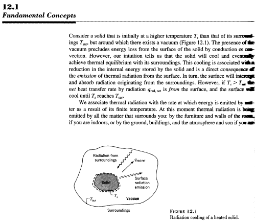
So lastly, we return to Kramm & Dlugi, and their “not even tiny point”, which nevertheless makes a useful point. They don’t provide a diagram, they provide an equation for energy balance at the surface – and I highlight each term in the equation to assist the less mathematically inclined:
Figure 5
The equation says, the sum of all fluxes – at one point on the surface = 0. This is an application of the famous first law of thermodynamics, that is, energy cannot be created or destroyed.
The red term – absorbed atmospheric radiation – is the radiation from the colder atmosphere absorbed by the hotter surface. This is also known as “DLR” or “downward longwave radiation, and as “back-radiation”.
Now, let’s assume that the atmospheric radiation increases in intensity over a small period. What happens?
The only way this equation can continue to be true is for one or more of the last 4 terms to increase.
So, when atmospheric radiation increases the surface temperature must increase (or amazingly the humidity differential spontaneously increases to balance, but without a surface temperature change). According to G&T and the illuminati this surface temperature increase is impossible. According to Kramm & Dlugi, this is inevitable.
I would love it for Gerlich or Tscheuschner to show up and confirm (or deny?):
Or even, which one of the above is wrong. That would be outstanding.
Of course, I know they won’t do that – even though I’m certain they believe all of the above points. (Likewise, Kramm & Dlugi won’t answer the question I have posed of them).
Hopefully, the illuminati can contact Kramm & Dlugi and explain to them where they went wrong. I have my doubts that any of the illuminati have grasped the first law of thermodynamics or the equation for temperature change and heat capacity, but who could say.
Read Full Post »