If you’ve just stumbled across this article without reading the earlier posts, please take a few minutes to review:
- Visualizing Atmospheric Radiation – Part One with a few basic concepts
- Part Two with some calculated spectra of upward radiation from the surface through to the top of atmosphere
Most people find the actual results of radiative transfer in the atmosphere non-intuitive. Intuition is not a good guide for this topic. So a lot of misconceptions arise because the results of atmospheric physics disagree with the mental models in people’s heads. Obviously the physics must be wrong or probably climate scientists haven’t understood the basics.. Shaking of heads.
For people interested in reality, read on.
We are still looking at how radiation travels and interacts with the atmosphere before anything changes.
There is a lot of fascination in the subject of the “average height of emission” of terrestrial radiation to space. If we take a very simple view, as the atmosphere gets more opaque to radiation (with more “greenhouse” gases) the emission to space must take place from a higher altitude. And higher altitudes are colder, so the magnitude of radiation emitted will be a lesser value. And so the earth emits less radiation and so warms up.
This “average height of emission” is often supplied as a mental model and it’s a good initial starting point.
Here is the result of the atmospheric model created with a surface temperature of 288K (15°C), 80% humidity in the boundary layer and 40% humidity above that (the “free troposphere). This is a cloud-free sample – clouds are very common, but really make life complicated and we are trying to provide a small level of enlightenment. Simple stuff first.
The model is the same as in Part Two – but with 20 layers instead of 10. More layers just means better resolution plus a little bit more accuracy. Each layer contains roughly the same number of molecules (same pressure differential between each layer), so each higher layer is progressively thicker.
The graph shows how much radiation (“flux”) makes it from the surface and from each atmospheric layer in the model to the top of the atmosphere (TOA) – [update Jan 9th, see revised graph in comments].
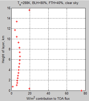
Figure 1
And here we’ve zoomed in by expanding the x-axis:
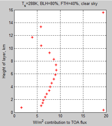
Figure 2
The TOA flux = 239.5 W/m², so what is the level where half of this value comes from below and half from above?
If we include the surface and the first 5 layers we don’t have quite half (48%), and if we go to 6 layers we get just over half (51%). Layer 5 is centered at 1.9km with the top of this layer at 2.1km. Layer 6 is centered at 2.4km.
So let’s say the “average” height of emission to space is just over 2 km (in this example).
There’s probably a better mathematical way of expressing it (this is more like the “median height”) but in fact this “average emission height” is really a curiosity value number anyway. In the words of guru commenter Pekka Pirilä (on another topic):
Any number that is not observable and that’s not used as an input or intermediate value in any calculation that aims to produce observable results is of curiosity value only by definition.
So it’s interesting but you don’t find it a key subject of any climate science papers. Still, being as so many people find it fascinating we will see how it changes as “greenhouse” gases vary in concentration and temperature profiles change.
While we are looking at this, let’s see what wavenumbers from what levels make the largest contribution to the TOA flux. That is, let’s look at the spectral distribution vs height.
First the TOA spectra for these conditions (Ts=288K, Boundary layer humidity=80%, Free tropospheric humidity=40%):
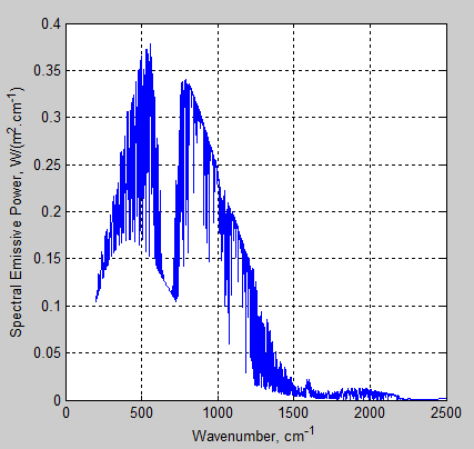
Figure 3
Now to see where this all originated from we divide up the wavenumbers into bands of 100 cm-1, and we see the contribution to the TOA flux by band and height in the atmosphere (note that height in km is now ‘lying on the side’ to the left and wavenumber to the right, lost the axes labels somewhere along the way):
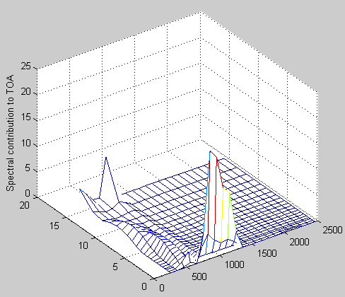
Figure 4
Zooming in a little:
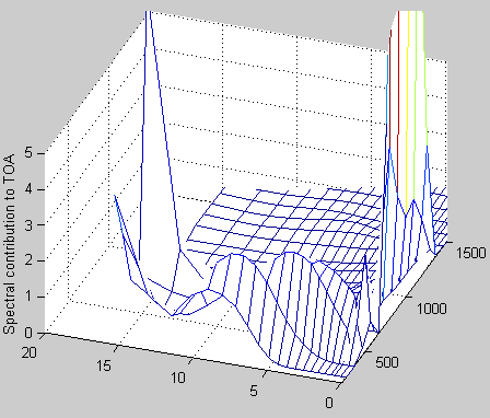
Figure 5
We see that in the “atmospheric window” between 800 cm-1 to 1200 cm-1 the surface transmits almost “straight through” (62% of surface flux makes it straight through to the top of atmosphere in this wavenumber range). A small component comes from around the center of the CO2 band (667 cm-1) from the top layer. The rest mostly comes from the “wings” of the CO2 band and where the water vapor absorption is not so strong, around 400 cm-1.
Conclusion
Hopefully seeing the actual data in these different ways helps to see that “average height of emission” is not a real concept or a particularly useful concept. Perhaps it’s a bit like averaging the kg of food consumed per day per person in the entire world. You get a value but the components that made it up are so wide ranging the average has lost anything useful. It’s not like average height of male 20-year olds in Latvia.
Transmission and emission of atmospheric radiation is extremely wavelength dependent.
Related Articles
Part One – some background and basics
Part Two – some early results from a model with absorption and emission from basic physics and the HITRAN database
Part Four – Water Vapor – results of surface (downward) radiation and upward radiation at TOA as water vapor is changed
Part Five – The Code – code can be downloaded, includes some notes on each release
Part Six – Technical on Line Shapes – absorption lines get thineer as we move up through the atmosphere..
Part Seven – CO2 increases – changes to TOA in flux and spectrum as CO2 concentration is increased
Part Eight – CO2 Under Pressure – how the line width reduces (as we go up through the atmosphere) and what impact that has on CO2 increases
Part Nine – Reaching Equilibrium – when we start from some arbitrary point, how the climate model brings us back to equilibrium (for that case), and how the energy moves through the system
Part Ten – “Back Radiation” – calculations and expectations for surface radiation as CO2 is increased
Part Eleven – Stratospheric Cooling – why the stratosphere is expected to cool as CO2 increases
Part Twelve – Heating Rates – heating rate (‘C/day) for various levels in the atmosphere – especially useful for comparisons with other models.
References
The data used to create these graphs comes from the HITRAN database.
The HITRAN 2008 molecular spectroscopic database, by L.S. Rothman et al, Journal of Quantitative Spectroscopy & Radiative Transfer (2009)
The HITRAN 2004 molecular spectroscopic database, by L.S. Rothman et al., Journal of Quantitative Spectroscopy & Radiative Transfer (2005)


Very nice. Cold you set water vapor to zero?
See Visualizing Atmospheric Radiation – Part Four.
So only the central line of the CO2 absorption band remains opaque up to ~ 15 km, but the important side bands within the CO2 13-17 micron band radiate to space from low down in the atmosphere and then peak at around 4 km . This agrees almost exactly to what I calculated – see graph here.
So I think Pekka Pirilä is missleading when he implies that most radiation in the 15 band originates from the stratosphere. Most radiation is actually from the lower troposphere peaking around 4 km above the surface, and surprisingly about 5% comes from the surface.
Clive,
I have said it clearly that my comment was about the wavelengths of strongest absorption. Extending the analysis down to 13 µm is highly misleading as that’s already in the region of the atmospheric IR window as you can see from SoD’s Figure 2 in Part Two. The absorptivity of CO2 is down by a factor of more than 10000 from the peak at 13 µm.
According to SoD’s calculation the stratosphere appears to be fully opaque over the range 645-695 1/cm or 14.4-15.5 µm and perhaps a little beyond that. You should not choose the range to include the really weak tails.
The range I give above is based on the uppermost layer of Sod, but the second layer from top is also fully within the stratosphere. Based on that the range of full opacity extends to 640-700 1/cm or 14.3-15.6 µm and almost full opacity to 625-715 µm or 14.0-16.0 µm. That’s about as far as it’s justifiable to extend the analysis of the 15 µm peak.
Pekka,
I don’t think that is completely true. Take a look at the absorptivity from the lecture notes ofCabellero here and then also take a look at a real IR spectrum from space here. I also have some doubts about the details of SoDs spectrum in fig 2, because (unless I am mistaken), it doesn’t include doplar broadening, (nor radiative transfer from lower levels ?). It is a valiant piece of work but the shape doesn’t quite reproduce experimental data.
So, Yes 13-17 microns cover the edges of the CO2 band, and below 13 microns is more or less the IR window. However the plank spectrum is ignorant of all this and more radiative flux passes through the shoulders than through the central line. As a result the radiation escaping to space between 13-17 microns originates from a wide range of heights in the atmosphere.
If CO2 increase then the effective height increases and OLR decreases assuming constant T and lapse rate. What surprised me is that if CO2 decreases then atmospheric OLR also decreases. Radiation from the surface increases exponentially and dominates below 100ppm. Another way of saying the same thing is that the IR window widens.
Clive,
Ir’s clear that the model of SoD is not complete and fully realistic. He tells that clearly in his post. Using the Lorentz line shape that cannot handle Doppler broadening is just one of the limitations. As far as I understand there’s no attempt to compensate for that by changing the line width from the collisional value. Thus the lines are too narrow at high altitudes. That increases transmission but cannot make much difference when the whole line is too weak as the absorption lines are close to 13 µm. If those wavelengths are calculated correctly we have, indeed quite a lot of radiation from the surface to space. On the other hand the band width used in the calculation causes “numerical broadening” that may lead to significant opposite errors in the results at altitudes where the lines are narrow in comparison with the band width.
The strongest absorption lines of CO2 at wavelengths around 13 µm by a factor of 10000 weaker than the main line. Only a logarithmic plot may make anyone think that such a weak tail can be considered a significant part of a broad absorption peak that’s formed from the main peak and the side peaks related to the rotational states. At 14 µm the lines have still a strength that’s almost 1% of the main peak. That’s enough to make the stratosphere as a whole rather opaque.
More accurate calculations of the transmissivity of the stratosphere require the use of Voigt line shape and very narrow bands in calculation because the lines are so narrow and the absorption minima between the lines deep. Lacking data from such calculations I cannot say much more about the outcome.
Off hand Eli has to agree with Clive. As one rises from the tropopause in the stratosphere the temperature increases, thus one would see a sharp upward going spike in the emission spectrum
http://rabett.blogspot.com/2009/12/answer-to-puzzler-couple-of-days-ago.html
Chris Colose gives a simple model of the greenhouse effect using the formula:
Ts ~ Te + Γ H,
where Ts is the surface temperature, Te is the effectuve temperature of radiation to space, Γ is the lapse rate, and H is “the flux-weighted mean altitude of the emission to space”, ie, the effective altitude of radiation to space. It is, to my knowledge, the simplest model of the greenhouse effect that includes both of the essential elements determining the surface temperature, and unlike other simple models used for teaching, does not encourage the misunderstandings that so commonly beset blog climate science.
My point is that using Pekka Pirilä’s definition that, it turns out that H is used as an intermediate value to produce observable results (Ts), and hence is not just of curiosity value.
Granted, it is only used for teaching, and to derive first order approximations of Ts – but that is still sufficient reason for the value to be of genuine interest.
Tom,
There was a post here on the same subject by Leonard Weinstein that got a lot of attention.
This post was derived from post at The Air Vent by the same author.
Please, let’s not reopen that discussion in this thread. I believe comments are still active on Leonard’s post here.
SOD: Could you explain why the lowest level in the atmosphere emits 20 W/m2 to space while the next layer above emits only 1 W/m2? There shouldn’t be a big temperature or composition difference between these two layers (unless water vapor decreases surprising fast with altitude) and the lower layer must travel slightly further to reach space.
Frank,
Well spotted.
The code is not well-written here. The value of transmitted flux is correct but the reason is bad. This one layer is quite thin.
The program divides the atmosphere up into equal Δp – to get similar numbers of molecules per layer. But I realized that if I had a “boundary layer humidity” and a separate “free tropospheric humidity” then changing the number of layers would alter this bottom layer and skew the results.
So I implemented a parameter called boundary layer pressure, which so far has been set to 920hPa (it can be altered when calling the routine).
The program should have been altered to produce equal pressure changes for n-1 layers above the boundary layer. But this is not the case. In the 20-layer example above, the pressures of the 21 boundaries are, in 103hPa:
1.0000 0.9197 0.9075 0.8624 0.8160 0.7708 0.7248 0.6794 0.6330 0.5876 0.5420 0.4960 0.4501 0.4042 0.3586 0.3130 0.2673 0.2215 0.1755 0.1298 0.0841
Which also highlights the fact that I changed the surface pressure from 1013 hPa to 1000 hPa as a temporary measure to make it easier to confirm that the way the program was creating pressure layers boundaries was correct. And haven’t yet changed it back.
Just finishing off another article with water vapor changes then I will be cleaning up the comments in the code and publishing so people can spot any gaffes.
Frank,
I fixed up the code so that the layers are equal pressure difference.
Here is the revised 20 layer model:
And here is the zoomed in section:
And the revised pressures and heights of the 21 boundaries are, in hPa and meters:
Pb zb
1013 0
919 810
873 1240
828 1670
782 2130
736 2610
690 3120
645 3650
598 4220
553 4820
507 5470
461 6160
415 6910
370 7730
324 8640
278 9660
232 10820
187 12190
141 13930
95 16360
49 20430
SOD: I haven’t been able to master the large number of posts you have put out since the beginning of the year. I returned here today trying to understand one of your more recent posts.
If I understand correctly, you are telling me that the lowest 5% of the atmosphere emits 22 W/m2 of radiation that makes it through the TOA while the second lowest 5% of the atmosphere emits only 6 W/m2 through the TOA. This is partly because the lowest 5% of the atmosphere is considered to be the boundary layer with 80% relative humidity and most of the layers above are considered to be free troposphere with 40% relative humidity. (I think I read elsewhere, that the rest is stratosphere with a fixed 6 ppmv.)
If water vapor were the only significant GHG in the lowest layers and given twice as much water vapor in the boundary layer, I expect twice as much emission from water vapor, not four times as much, attenuated to some extent by the absorption of the water vapor above as seen in layers 3, 4, 5, 6 etc., which are gradually increasing their effective emission with altitude through the TOA despite being colder. So I would have predicted something like 10 W/m2. (Given that CO2 contributes some emission and it’s mixing ratio doesn’t change across the boundary layer, 10 W/m2 is an upper limit. If half of the emission escaping from the lowest layer through the TOA actually came from CO2 (unlikely), then I’d have predicted 7.5 W/m2.)
Looking at the column labeled zb (altitude?), however, the bottom layer is twice as thick as the next layer – which contradicts my understanding that each layer contains the same weight of atmosphere.
Your assumption that there is a sudden discontinuity between the relative humidity in the boundary layer (80%) and the free troposphere (40%) may be approximately correct in the descending regions of the subtropics, but is unlikely to be realistic for the global as a whole. If you ever want to make changes to the model, using measured absolute humidities might be preferable.
I’m not sure how your program handles the water vapor continuum. Most of the continuum appears to be water vapor dimers. If water vapor monomer concentration drops by a factor of two (as you move higher in the atmosphere), then dimer concentration drops by a factor of four.
Frank,
If I made the bottom layer (the boundary layer) of variable height then changing the number of layers would be guaranteed to change all the radiative transfer calculations due to the different humidity in boundary layer and free troposphere. So it’s kind of a compromise.
So in this version of the model the boundary layer is 80 hPa thick, while the next layer is 46 hPa thick.
So we have twice the number of molecules in layer 1 vs layers 2,3,4,etc.
The continuum is a function of the square of the concentration of water vapor molecules.
So – if the temperature was constant with height – the boundary layer with 80% relative humidity would have 4x the continuum effect of the next layer up with 40% relative humidity. And the bottom layer is twice as thick so it would have 8x the effect of the next layer up.
In reality the boundary layer is at a higher temperature which increases s.v.p so the concentration of water molecules is increased by more than than a factor of 2.
So the effect of the continuum will be a factor of say 10x lower in the 2nd layer vs the boundary layer.
As you point out, the continuum is only one part of the whole story.
We could check – I should rerun some models and separate out the effects from the different GHGs and the continuum.
This is spot on. The only reason for doing it this way is to allow a simplification – but not too simple.
Later on in Part Twelve – Heating Rates I have some standard AFGL atmospheres using the specified water vapor, ozone, CO2, etc.
I will almost no time over the next week, but next opportunity I will rerun those std atmospheres and post the graphs of TOA contribution from each level.
I had the chance to squeeze this in..
Here is the AFGL Tropical atmosphere. As suggested by Ebel, I changed the code to plot cumulative contribution from each layer:
There are more layers in this model – it just uses the values provided (temperature, humidity, etc) for every 1km in the atmosphere. So each layer has the same vertical depth.
This means (when using the standard AFGL atmospheres) that the pressure difference for each layer is not constant.
And here in contrast is the AFGL Subarctic winter:
The total TOA flux is 192 W/m2.
We can see that the surface contribution to TOA is higher – because the atmosphere transmits more.
For reference, here is the AFGL Subarctic winter profile:
The AFGL Tropical profile:
SoD and Frank,
I have played quite a lot with the model as well and all simplifications and assumptions have clear justifications. Working with the model myself I have also fair understanding of what the graphics is about. Thinking a little more about the graphs I notice that many of them have been misleading. The the observations of Frank and the improvements in the new graphs tell on the nature of these problems.
In some cases a cumulative distribution would avoid the problem and present the facts well enough, in some other cases dividing the values by the mass of the layer would be an improvement, when the masses are not equal as they cannot be, when stratosphere is studied in more detail.
One more set of graphs that I find badly misleading are those of the part nine, which tell about reaching the equilibrium. The whole dynamics shown in that part is just an artifact of the computational method rather than dynamics of any atmosphere (plus ocean), real or idealized. This is due to the way the model iterates the development of the temperature profile. The results depend on the number of iterations for each time step. Using a very large number for each time step gives the same results as my modified code that avoids the iteration totally. With the small number of iterations the little dynamics present in the atmosphere and ocean is overwhelmed by the very strong one brought in by the method.
There are certainly many other examples where working with the model and knowing, how the graphs should be interpreted, makes it difficult to notice, how misleading they are to others.
Hi SOD, I know these are very old posts but there are two things I’m curious about with the model and your graphs.
Firstly, the contribution of the transmitted flux at around 18kms has increased considerably (and appears to be increasing) but doesn’t seem to be reflected in your cumulative graph.
Secondly, if the contribution is increasing at 18kms, shouldn’t you plot out to much further? At least to 50kms at the top of the Stratosphere?
I mean if you only plot the transmitted flux in the Troposphere, then the ERL can only live in the Troposphere, right?
As a followup and on reflection, I’m assuming the transmitted flux value at 18kms is actually the value “above” 18kms. I’m surprised the stratosphere isn’t contributing more to the OLR as its warmer. Something seems off.
TTTM,
Yes, the stratosphere is warmer, but there’s not much mass there and almost no water vapor. You can see a spike in the center of the CO2 dip from CO2 emission in the stratosphere, but that doesn’t contribute much to total emission. If you look at Archer’s MODTRAN model page, you can see the difference. For example, for the Tropical Atmosphere at 17 km (stratopause) looking down, the upward radiation at 299.4 W/m² is higher than the upward radiation at 70km looking down, 298.5 W/m². Some of the upward radiation at the troposphere is absorbed in the stratosphere and the emitted radiation doesn’t make up for it.
The radiation at the TOA is not the result of the transmission, but the average value of the temperatures of the pressure geometrical heights or heights from which the radiation reaches the space. Radiation that was emitted from deeper layers is largely absorbed again and does not reach, therefore, the space.
The radiated power from heights where no more radiation from deeper layers is absorbed, is determined from the Planck function corresponding to the temperature.
As illustration should be more useful a cumulative frequency curve, where in the X-axis is the sum of the radiation power and the y-axis the corresponding heights up to which this sum is reached. It’s clearer than the individual contributions of each layer and it can increasing the number of layers without substantially the clarity is lost.
Scienceofdoom,
“If we include the surface and the first 5 layers we don’t have quite half (48%), and if we go to 6 layers we get just over half (51%). Layer 5 is centered at 1.9km with the top of this layer at 2.1km. Layer 6 is centered at 2.4km”.
For pure curiousity value:
Employing a very different method I estimate the effective emission altitude at 1.9km, the effective emission temperature at 276K and a GHE magnitude at 12 degrees C. The result is based on surface emissivity of 0.93 and atmospheic emissivity proportional to the square of temperature.
How can I post the sum curve? As email, but with what address?
You could create a JPG or PNG of your graph using Paint, upload to a photo hosting service and post a link. That’s what most of us do.
Ebel,
That’s a very sensible approach. I’ll update the code and plot cumulative values for future graphs.
[…] a look at Part Three – Average Height of Emission and Part Four – Water Vapor for more […]
[…] Part Three – Average Height of Emission – the complex subject of where the TOA radiation originated from, what is the “Average Height of Emission” and other questions […]
[…] Part Three – Average Height of Emission – the complex subject of where the TOA radiation originated from, what is the “Average Height of Emission” and other questions […]
[…] Visualizing Atmospheric Radiation – Part Three – Average Height of Emission Visualizing Atmospheric Radiation – Part Five – The Code […]
[…] Part Three – Average Height of Emission – the complex subject of where the TOA radiation originated from, what is the “Average Height of Emission” and other questions […]
[…] Part Three – Average Height of Emission – the complex subject of where the TOA radiation originated from, what is the “Average Height of Emission” and other questions […]
I have been working on a different approach to calculating the effective emission height for CO2 in the atmosphere. Instead of calculating radiative transfer from the surface up through the atmosphere to space, I decided to do exactly the opposite. IR photons originating from space are instead tracked downwards to Earth in order to derive for each wavelength the height at which more than half of them get absorbed within a 100 meter path length. This identifies the height where the atmosphere becomes opaque at a given wavelength. This also coincides with the “effective emission height” for photons to escape from the atmosphere to space. I wrote a program to do this using a standard atmospheric model and a line by line calculation for CO2 absorption using data from the HITRAN spectroscopy database. The effective emission height looks like this.
I have also written this up here and used the result to estimate the radiative forcing caused by a doubling of CO2. I get 3.5 watts/m2
Clivebest,
Have you taken the Voigt profile into account. It’s likely to have a significant influence near 667 1/cm and some influence over the range from 645 to 690.
As you notice, your results are closely related to those of SoD. Your graph is a nice way of presenting this particular point, while the same physics is taken fully into account in SoD’s model.
I must admit that I don’t fully understand the Voigt profile! The Fortran program uses Lorentz function and integrates over multiple line overlap to calculate absorption cross-sections. For sure it can be improved.
I think SoD’s model is great. It inspired me to try another approach.
The basic idea of the Voigt profile is simple. In very rare atmosphere collisions are so infrequent that the related Lorentz profile is very narrow. Under such conditions the Doppler effect starts to be of similar importance. The Doppler effect alone would result in a Gaussian line profile from the Maxwell-Boltzmann distribution of the molecular velocities. The widths of the to profiles taken alone are comparable in the upper stratosphere. At lower altitudes the Doppler effect is insignificant and above the stratopause it starts to dominate. The most difficult range to calculate is that where the both effects are comparable. There the far tails are given by the Lorentz profile but the central peak is significantly broader and lower.
I found a paper that published Matlab-code for calculating the Voigt lineshape fast enough to make it practical. It’s certainly slower than calculating the Lorentz profile, but fast enough when applied with care only when it may matter.
Using the Voigt profile for the stratosphere makes little difference on any results that concern troposphere or surface. Thus it’s of interest only when we want to study what happens at altitudes of more than 30 or 40 km. Even significant changes at those altitudes have little influence on the radiative balance of the troposphere. If those changes do influence troposphere, that must happen trough other mechanisms related to the dynamic behavior of the stratosphere.
Reply to SOD February 24, 2013 at 2:12 am:
I’m confused when looking at the graph you posted of the cumulative TOA flux from various layers of the tropical atmosphere. The surface layer seems to be emitting about 30 W/m2 through the atmosphere – reasonably consistent with the 40 W/m2 in the KT energy balance diagram. The tropics are a little warmer than the global average used by KT and the atmospheric window is probably narrowed by the enhanced water vapor continuum in the humid tropics.
My problem arises when comparing the layers immediately above the surface to the surface. The surface emissivity in the tropics is mostly ocean, perhaps 0.97-0.99. Whatever the emissivity of atmospheric layers above the surface, I assume that it must be LESS than the emissivity of the surface because there are some wavelengths where the atmosphere does have negligible emission. Unlike the surface, the atmosphere emits best at precisely the wavelengths it absorbs best. So my intuition suggest that it should be harder for the radiation emitted by these lowest layers to reach the TOA. Finally the temperature is dropping with the lapse rate, down 3 degC for the average of the first layer, down 10 degC for the second layer, etc. Those are roughly 1%, 3%, etc changes in temperature; and emitted radiation drops by the fourth power, roughly 4%, 12% etc. Despite these problems, each of the lowest layers of the atmosphere are contributing as much to the TOA flux as the surface. Above. we’ve discussed the graphs you’ve posted in your comment of January 9, 2013 at 10:12 pm. Those graphs show much less emission from the lowest layers of the atmosphere compared with the surface. It might be worth checking for a problem somewhere.
I recognize that the emissivity/absorptivity of a gas depends on the quantity of gas under consideration (and that it can never rise above 1). One set of graphs in question use layers measured in altitude; the other, pressure. When the thickness of a thin layer is doubled, the emissivity of that layer doesn’t double, because some of the radiation it emits is absorbed before it reaches the surface of that layer. Are your layers always thin enough to avoid this problem?
(FWIW, I prefer layers of constant pressure change, because they represent equal numbers of emitting molecules, except for the drying with altitude. Putting pressure on the left-hand vertical axis and altitude on the right-hand axis is the best of all world for those like me who need to stop and think about how to translate one into the other.)
Frank,
The strong dependence of the continuum absorption is probably enough to explain the importance of the two lowest layers for the emission from the tropical atmosphere.
.. absorption on the moisture is probably ..
Frank,
Interesting thoughts. I’m pretty sure the model is calculating radiative effects correctly from a number of perspectives, including the fact that the heating rates for model atmospheres are a close match with professional results.
But the whole point of this series is to test ideas and provide insight. Next weekend, when I am back in front of my (Matlab) PC I will provide some more detailed results:
a) emission from each layer
b) spectral emission from each layer
c) spectral emission from each layer that is transmitted to TOA
– and if that still leaves unanswered questions we can review what proportion of each layer’s spectrum gets absorbed in each layer above.
That’s the beauty of having a model where we can inspect the innards..
Frank,
I took the spectral emission from the surface and the lowest three layers, each 1km thick.
The emission is plotted, and the total flux is noted in the legend.
The second graph shows the TOA transmitted spectrum for each of those layers – on the same vertical axis, again with flux (transmitted TOA) noted in the legend. The graph can be expanded by clicking on it:
And the second graph on an expanded scale, again, click to expand:
You can see why it’s difficult to figure out in your head why the value should go up or down for each layer.
For a layer closer to the ground (vs a layer higher up) the emission will be higher (because temperature and water vapor concentration is higher), but the absorption through to TOA will be higher due to more GHGs above.
Which ones wins? As we see in the above graphs, the results vary for any given wavenumber.
If you want to see more layers or different layers I can easily produce those graphs. Any more specific request can probably be produced.
And here are the comparable results for the sub-arctic winter, click to expand:
And the expanded view of the transmitted TOA spectrum:
This one is probably easier to expect. The surface transmitted flux is much higher because the atmosphere has much less absorption. Therefore, the atmosphere has much less emission – and so the TOA transmitted flux from comparable atmospheric layers is much lower. However, it isn’t easy to predict whether the layer above or the layer below contributes more to the TOA transmitted flux because of the various competing effects – which vary with spectrum and temperature.
Pekka:
Each different method of presenting data can convey a slight (or sometime very) different message. The best graph or table is the one that provides the information or “picture” you are seeking.
The part of the “picture” that is missing for me is: What is happening to the photons? If I consider a thin slab of atmosphere (say 1 mb thick or 0.1% of the atmosphere) centered at a given altitude (say 1 km), what fraction of the photons emitted downward reach the surface and what fraction of those emitted upward reach space? Of those that are emitted downward (or upward) and are absorbed by the atmosphere, how far do they travel before being absorbed. There are obviously a wide range of distances traveled, so one might want to know something about that distribution: the shortest-most quickly-absorbed 5% travel an average distance of only 100? m downward, the next 15% travel an average of 250? m, the next 20% travel 400? m, the middle 20% travel an average of 700? m, and 30%? reach the surface. The best way to present this type of information would be a table.
Frank,
SoD’s model produces related information as optical depths of each layer for each wavelength in the sample. The table you are asking for could be calculated from these results and the temperatures that are also available.
Each of us looks at the same issues in different ways. Therefore the optimal set of information that we wish to have varies as well.
SoD,
Your figures 1 and 2 illustrate quite clearly why the common description of the greenhouse EFFECT is fraught with problems:
It states that you can find the surface temperature of say Earth by knowing its planetary (S-B calculated) BB emission temperature, its ‘effective radiation level’ (ERL), which by default is AT this particular temperature, AND the tropospheric lapse rate: T_sfc = T_erl + (h_erl * lr) -> 255K + (5.1 km x 6.5 K/km) = 288K.
But this makes no sense, because there exists no such level in the Earth system where the temp is 255K and the radiative flux to space is 239 W/m^2, as your figures evidently show.
So the whole concept of lifting the ‘radiative surface’ of Earth by putting more GHGs into the atmosphere can only support the AGW argument, not the original GHE argument. It doesn’t in itself explain why the surface of the Earth is warmer, in the first place, with a ‘radiatively active’ atmosphere on top than without. And especially not the size of the effect. Because what level do you draw the lapse rate down from? Radiation is just going out, to match the incoming, from ALL levels. It is a ‘total’ (accreted) flux (as your figures also show). Why, then, would it matter what the ‘average’ level is? The total is the total either way. Determined by 1) surface temperatures, 2) tropospheric temperatures and humidity, and 3) cloud cover.
I’ll tell you why. This is all about convective processes, not radiation. Convection governs the movement of heat from the surface to the tropopause (through the troposphere). The radiation is simply what rids the tropospheric heat to space and is simply a result of the 3 points above -> OLR at ToA. It is not a cause of anything. It just IS.
One of your original statements on this post, SoD, is the following:
“If we take a very simple view, as the atmosphere gets more opaque to radiation (with more “greenhouse” gases) the emission to space must take place from a higher altitude. And higher altitudes are colder, so the magnitude of radiation emitted will be a lesser value. And so the earth emits less radiation and so warms up.”
But this is a purely theoretical construct based on the assumption that radiation somehow controls temperature distribution in the troposphere. Evidently it doesn’t. Heating starts at the surface and is propagated by convection up along the lapse rate to the tropopause. That’s how the tropospheric temperature profile is set. The lapse rate doesn’t work downwards. The heat between surface and atmosphere doesn’t propagate downwards.
And the available data from the real world shows no sign of your suggested effect. Total OLR at ToA has rather increased than decreased over the last 30 years of mounting atmospheric GHG concentration.
It’s fine to have an hypothesis, but you need data from the real world to confirm it. The OLR data does NOT. They go a long way in contradicting it.
Your IR diagrams with those distinct CO2 bites don’t show what you think they show. All they show is that less energy goes out to space in the particular CO2 IR frequency band. That doesn’t mean that the energy doesn’t leave the Earth system, that it’s somehow ‘trapped’ within it. The atmosphere radiates to space based on bulk temperature, not on the specific spectral properties of its constituent gases. You know of course that the IR absorbed from the surface by the CO2 molecules is NOT reemitted at the same frequency. That’s not what we’re looking for. It goes into the total energy fund of the atmosphere, maintaining its temperature. Well, the temperature radiation of Earth doesn’t have anything to do with CO2’s or H2O’s spectral properties. It is a bulk property.
Kristian,
As I said in the conclusion of the article, the average in this case is not a particularly useful concept.
Let’s look at the total OLR.
The example I gave is one particular surface temperature, atmospheric temperature profile and GHG concentration profile. We have to pick one to work with to establish some basic points.
If we increase the CO2 concentration in the atmosphere then, for this specific example, what happens to the total OLR? Increase, decrease, or stay the same?
Thanks for replying, SoD.
But is this a question for me to answer? The whole point here is that I don’t agree with your fundamental assumption that the tropospheric GHG concentration profile matters at all. I think you have the whole thing backwards. The tail wagging the dog. Radiation in the troposphere just IS, a result, not a cause of temperature.
Convection is what moves heat through the troposphere, maintaining the temperature profile in the process, driven by surface heating. Radiation simply lets the Earth system rid its energy to space. It won’t do that to a LESSER degree with MORE GHGs in the atmosphere.
Can you please justify with some observational data from the real world how radiation and the GHG concentration profile would control surface and tropospheric temperatures?
The reason I asked the question is to establish whether we agree on absolute basics. From your answer I’m not sure.
Let’s accept, for the sake of argument, that this point is totally irrelevant.
But just to help me, why not tell me what you think. Same surface temperature, same atmospheric temperature profile, more GHGs: what happens to OLR?
Kristian,
Can you explain this statement. Is there an equation or principle you would use to quantify this or put some boundaries on it?
Because outgoing longwave radiation has different values at different locations and different times. What determines this value?
SoD, you ask: “Same surface temperature, same atmospheric temperature profile, more GHGs: what happens to OLR?”
If you read the last paragraph of my original comment, you would understand that I can’t see why this should affect TOTAL OLR at ToA at all. Also since OLR from the real-world data only shows signs of responding to surface temp, troposphere temp + humidity and clouds, you would have to somehow set the premise that the radiative properties of GHGs affect or even control one or more of these variables, leading secondary/indirectly to an OLR effect. That’s your basic assumption, that since the ‘mean’ radiation have to occur from a higher, and hence colder, level, then everything below it will be forced to warm, because less goes out FROM THIS HIGHER ‘MEAN’ ELEVATION. Energy from the surface is thus somehow ‘trapped’. That is quite an assumption, seeing that we know that the surface itself and the entire atmosphere (all layers) at all times help and contribute to radiating Earth’s TOTAL flux to space, the flux measured as coming out of the ToA, not the ERL (the 255K layer). And also knowing (all data shows it) that the surface always warms first from where the heat propagates UPWARDS along the lapse rate, setting the tropospheric temperature profile from below.
Yours is an extraordinary claim that requires extraordinary evidence (from the real Earth system). I can’t see that anyone of you has ever provided anything remotely resembling such evidence, that the lapse rate is perturbed first at altitude, that warming can propagate from the atmosphere down to the surface – the atmosphere will have to warm first, reducing the temperature gradient going up through the air from the surface, in order for energy to pile up at the surface so that THIS can warm. How is this going to happen in an open atmosphere? And where is the observational data pointing to such a process occurring on any level?
Once again, this isn’t about radiation at all. It’s about convective processes. About the workings of gases in a gravity field heated from below. Radiation is a result of temperature, not a cause of it.
Can I explain this statement?
Yes. The main job of the GHGs is to make the atmosphere able to rid itself of the energy it receives from the surface (and the Sun). It is NOT to make the atmosphere able to warm. The atmosphere would’ve warmed with or without GHGs. Through other mechanisms than radiative transfer. It could however not COOL effectively to space without GHGs. Because there are no other mechanisms available for that than radiation.
So which atmosphere is warmer? One with GHGs, absorbing energy as heat from the surface (and the Sun), distributing it along a set lapse rate profile, but ALSO releasing it efficiently to space, or one without GHGs, absorbing energy as heat from the surface, distributing it along a set lapse rate profile, but NOT able to adequately rid itself of it to space?
SoD, is your contention that an atmosphere with lots of GHGs in it is less well suited to cool to space than one without any?
Kristian,
In response to my question:
You replied on March 10, 2014 at 7:46 pm:
This is very interesting because it is at odds with basic radiative physics.
You can see equation 11 in Understanding Atmospheric Radiation and the “Greenhouse” Effect – Part Six – The Equations:
dIλ/ds = nσλ.(Bλ(T) – Iλ)
in words this says that the change in monchromatic intensity as the radiation travels through the atmosphere is a function of:
– n, the number of molecules (of each type)
– σλ, the capture cross section at that wavelength, which is measure of the molecule’s absorptivity
– the difference between blackbody emission (at that temperature and wavelength) and the intensity of radiation
Therefore, basic physics explains that if the local temperature is lower than the temperature of origin of the radiation then dIλ/ds will be negative – radiation will reduce in intensity. If the local temperature is higher than the temperature of origin of the radiation then dIλ/ds will be positive – radiation will increase in intensity.
And basic physics explains that for σλ > 0 (absorption at this wavelength), increasing n increases this change.
So for an atmosphere which gets colder with height, upwards radiation reduces in intensity (if σλ > 0) and as n increases dIλ/ds gets more negative.
Therefore, increasing the concentration of a GHG will reduce OLR for the same surface temperature and atmospheric temperature profile.
(For the same reasons, downwards radiation increases in intensity with more GHGs).
For this to be wrong, then the Beer-Lambert law of absorption would have to be wrong, or Planck’s law of emission would have to be wrong (or both). All the textbooks on radiative physics would need to be rewritten.
Please can you explain what is incorrect about the above equation, or the above explanation of the consequences of this equation.
And you added:
How do you think humidity affects OLR?
Of course, I believe humidity affects OLR because water vapor is a GHG, and I believe more humidity reduces OLR given the same surface temperature and atmospheric temperature profile.
This is exactly the same effect I wrote in the first part of this comment.
Following my comment from March 10, 2014 at 8:41 pm – which should be addressed first as it contains proof of one fundamental premise..
As explained in my last comment, I rely on basic physics well-known for 100 years and turned into the theory of radiative transfer since at least 1950 by Nobel prize winning Subrahmanyan Chandrasekhar.
OLR does decrease with more GHGs, for the same surface and atmospheric temperature. DLR increases under the same conditions.
As already explained in the article I don’t particularly like the “mean elevation” explanation. It’s just a concept to help people with a mental model.
Let’s dispense with possibly illuminating models and instead stick with basic physics – the equations.
The equations as demonstrated show that more GHGs, for the same surface temperature and atmospheric temperature profile, will reduce OLR.
If we assume some kind of steady state condition prior to the GHG increase, i.e., absorbed solar = OLR, then more GHGs, less OLR means that the troposphere must warm.
This is an inevitable consequence of the first law of thermodynamics.
As the troposphere warms, OLR increases. Eventually a new steady state results at a higher surface temperature.
This is all without feedbacks.
Energy is not “trapped”. It’s a turn of phrase often used to help people with mental models. Let’s again dispense with ideas that might or might not help conceptually.
The balance of this statement is completely correct – starting from “seeing that we know..”
Perhaps after you have addressed the earlier points we can continue reviewing your other statements.
Kristian,
A very good question.
An atmosphere with no GHGs cannot cool to space at all (because it cannot radiate). At atmosphere with GHGs can cool to space.
And in fact, the more GHG’s, the more the atmosphere radiates (cools) to space.
After you respond to my earlier comments (responses to your earlier points/questions) we can pick this one up so that we can see what the implications are.
After being banned from “And Then There’s Physics” Kristian sent me a email presenting similar views. Part of mys answer follows. I hope it saves some futile effort from others who consider answering the above comment.
Albert Einstein famously stated: “If you can’t explain it to a six year old, you don’t understand it yourself.”
He might have added: “If your ‘simplified’ explanation to the public isn’t how it really works, it is simply wrong and illogical and unphysical, then it’s pretty clear you’re trying to cover something up by still pushing this ‘simplified’ explanation in front as a red herring. It’s all about smoke and mirrors.”
And what you’re covering up is of course that you have no real mechanism, only vagueness and appeals to ‘complexity’ (like Al Gore said, ‘It’s complicated’), it’s all (including your ‘calculations’) based on flawed assumptions and circular reasoning (I know you don’t see it, Pekka). Reality always trumps theory. And reality simply doesn’t confirm your ‘hypothesis’.
All you have is a purely theoretical construct. That isn’t seen and couldn’t work in the real Earth system.
Kristian,
You are at odds with very many. All those think that the points are simple and that they have been explained to you many, many times. When you refuse to accept the simple explanations, and when you presented many points correctly in your email to me, I tried to continue from that. I made my explanation to address directly the point, where your ideas started to deviate from the well known physics.
Now we have the situation that you don’t accept simple and fully valid answers, and you don’t accept an answer that’s custom formed to address your own description.
When this kind of failures of explaining the basics to you have repeated themselves so many times, it starts to be clear that getting the points clarified through a net discussion will not work.
You have understood so much of the physics that you should understand these points as well by going more carefully through the sources that you must already know.
If it would be only me against you, you would be right to think that I may be in error and you right, but when you have seen the same with so many, you should accept that the error is in your thinking.
There’s no “hypothesis” in what I have written, it’s certain in the sense the word “certain” is commonly used.
See, Pekka, this is my problem with your kind. You just know best. Not willing (or capable of) seeing your own position from outside your bubble. You’re simply not arguing. You just go la-la-la-la to any opposing argument and then return to your talking points. Your version, your understanding. Not willing to even contemplate that there might be other versions, other understandings that would ALSO work theoretically.
You’re just TELLING (The ‘Listen and shut up! I understand this! You don’t!’ approach). You’re not addressing, not willing to address, a single specific counter-point. This lowers the credibility of your own argument. Why is it so hard to address points directly? Why do you feel this endless need to evade?
The point is, Pekka, don’t mind if I’m ‘at odds with many’. Read what I’m actually saying. The points I’m making. Try to relate to it. Without misrepresenting them. Try to lift your eyes beyond the tip of your nose.
Kristian,
There’s one major difference between our views. Mine agrees with very many very competent people, yours does not. That’s not the only reason for my trust, but that’s an essential part of that.
Scientific knowledge is not absolute, but it’s to a major part solid. It’s important to avoid overconfidence but it’s also important to have confidence when that’s based on strong arguments. Doubting everything would stop progress as effectively as unjustified dogmatism.
I’m not doubting ‘everything’, Pekka. I’m calling out vague nonsense arguments when I see them. That goes for warmist and skeptic arguments alike. I have no affiliation. I just want to find the truth about how the world works. I’m not skeptical to the ‘well-accepted’ GHE explanations (for there are several) out of ideology. I just want real, open science to be practiced without prejudice. I want people to look at the data, what the world is telling us, without resorting at once to one’s own inherited preconceptions and a priori assumptions to ‘explain’ it at every turn.
And my alarm bells go off as soon as someone is trying to make arguments out of authority and numbers, taking the high road, not being willing to defend his or her position with actual scientific arguments, rather insinuating or stating flat out that I should just keep silent, because ‘everyone agrees on this’. ‘The science is settled.’ ‘The debate is over.’ What debate? Was there ever any scientific debate? The conclusion was already there from the beginning. That is NOT how science ought to work, Pekka.
Kristian,
You wrote in one of your comments:
That’s exactly the opposite of what physics tells. This has been told you by many. If you refuse to accept this kind of basics, it’s very difficult to proceed.
OK, Pekka, I will ask you the same question as I did SoD:
Is it your contention that an atmosphere containing GHGs is less well suited at cooling to space than an atmosphere without any GHGs?
Your constant appeal to authority and numbers (‘This has been told you by many’) and nothing else, makes you an uninteresting opponent.
Kristian,
What’s warming or cooling is the Earth as a whole. The rather constant lapse rate forces the surface and the troposphere warm or cool in unison. Therefore the right question concerns the cooling of the whole Earth including both the surface and the atmosphere, when both the surface temperature and the GHG concentration are varied.
For a fixed surface temperature an Earth without any GHGs or very little GHGs cools most efficiently to space, because nothing stops the radiation from the surface on the way out.
When you add GHGs less and less radiation from lower altitudes (icluding the surface) passes through a layer of atmosphere. That reduction is larger than the addition from radiation emitted by that layer, when the layer is colder than what’s below.
Therefore the Earth surface warms the more the more GHGs there are in the atmosphere.
But, Pekka, I would very much like to see SoD answer my first posting. Not you. Because you’re not replying. You’re just telling. You’re addressing anything of what I’m pointing to. Simply repeating your talking points.
Maybe SoD could give the REAL explanation as to why the surface of the Earth is 33K warmer with an atmosphere with GHGs than without GHGs. One that is physically and logically coherent, not just a random string of words that are meant to convey a sense of ‘sciencyness’.
Sorry, “you’re NOT addressing anything of what I’m pointing to.”
Sorry, SoD, my quarrel with Pekka ends here.
Ich schreibe diesen Beitrag auf deutsch – vielleicht übersetzt jemand den Text (I write this post on German – maybe someone can translated this text).
Wie ist die mittlere Höhe der Abstrahlung zu definieren? Da gibt es verschiedene Möglichkeiten. Deshalb noch mal die Abschreibungsverhältnisse beschreiben: Emittiert wird in der ganzen Höhe – die Abstrahlung aus tieferen Schichten wird absorbiert, je kürzer die Absorptionslänge bei einer bestimmten Wellenlänge ist, um so weniger der Emission aus tieferen Schichten erreichen das All.
Beimehr Treibhausgasen verändert sich nicht nur die Absorption, sondern auch das Temperaturprofil der Atmosphäre, wodurch das Spektrum ins All nicht nur von den Absorptionslängen abhängig ist, sondern auch vom Temperaturprofil. Sehr schön ist das am Spectrumverlaauf um 15 µm zu sehen: Die Absorptionslänge ist bei 15 µm am geringsten und wird mit zunehmenden Wellenlängenabstand immer größer. In der Mitte ist die Absorptionslänge so kurz, daß sie nur bis in die warme Ozonschicht reicht. Mit zunehmenden Wellenlängenabstand reicht die Absorptionslänge immer tiefer in die Stratosphäre hinein – aber weil die Temperatur in der Stratosphäre fast konstant ist, folgt die Intensität des Spektrums fast dieser Temperatur. Wird die Absorptionslänge noch größer reicht sie zunehmend in die Troposphäre hinein, wo es immer wärmer wird, d.h. die Intensität steigt.
Was will man da als mittlere Emissionshöhe definieren? Mit der „mittleren“ Emissionshöhe hängt der Übergang von der Stratosphäre in die Troposphäre zusammen (Schwarzschild-Kriterium). Ich würde deshalb keine mittlere Emissionshöhe definieren, sondern eher die Frage beantworten: „Wie ändert sich der Tropopausendruck mit zunehmender Treibhausgaskonzentration?“ Die geometrische Höhe ist dafür wenig geeignet, da sich bei Temperaturänderungen durch Ausdehnung die Dicke der Troposphäre ändert, ohne das sich der Tropopausendruck ändert.
MfG
Ebel,
I don’t translate any of your text to English, but I hope that the answers indicate well enough also the questions.
You ask, how the mean height of emission is defined. I don’t think that it has been defined at all. What people discuss is the effective height of emission, which is a somewhat different concept than the word “mean” or “average” or “mittlere” in German implies. The effective emission height has an indirect definition that requires two steps:
1) The effective radiative temperature is defined as the temperature of a black body of the same size that radiates as much IR as the Earth. In a stationary state that amount must be (very close to) equal to the solar radiation absorbed by the Earth. With the present albedo that temperature is 255 K.
2) The effective radiative height is the altitude, where the temperature is equal to the effective radiative temperature (255 K or a little different with a different albedo or in an out-of-balance state).
That’s all. The effective radiative altitude is nothing more, only the result of the above calculation. Nothing specific can be observed at that altitude as a local property. The amount of upwards radiation is not required to have any particular value at that altitude.
I have done some calculations using the radiative transfer model of SoD that forms the basis of this series of posts. The results are seen in this figure. The lowest cyan curve tells, what percentage of the IR radiation that exits at the top of the atmosphere originates from altitudes below a given height. We see that about 37% originates below the whole atmosphere, i.e. from the surface, and 50% from below 2.5 km. Those numbers apply to the clear sky case of the U.S. Standard atmosphere with 400 ppm CO2. That’s not representative of the whole atmosphere, but serves well for the exercise.
The red curve is otherwise the same, but with 800 ppm CO2. The green and blue curves tell similar results for a narrow band of wavenumbers (719-769 1/cm, corresponding to 13.9 µm and 13.0 µm). This is one of the bands where the influence of additional CO2 is greatest. The influence is furthermore large also below 12.5 km, which is the tropopause level of this standard atmosphere.
Looking again at the cyan and red curves, we see that the red curve is at a height 200 – 500 m higher in the troposphere. The effective radiative altitude must go up by a similar amount (a little less as only a small fraction of emission from surface moves up). What the curves do above 12.5 km has little influence on the energy balance of the lower atmosphere and surface.
In a sudden addition of CO2 the temperature of the lower stratosphere is not likely to change much. The upper stratosphere cools quite strongly, but the lower probably not. Thus the tropopause is likely to move up at this stage to join the temperature trend of the troposphere with the temperature of the lower stratosphere.
In the longer term, where the balance is restored trough warming of the surface and the troposphere, the tropopause reacts to the warming as well. It’s likely to get warmer, but not quite as much as the surface gets warmer. Thus it’s moves up a little from the original level, but almost certainly much less than the effective radiative altitude. What exactly happens to the tropopause, and what happens to the stratospheric temperature profile is a more complex issue.
What I describe above is more certain for idealized cases like those of the standard atmosphere, where the lapse rate of the troposphere is essentially constant and the lower stratosphere isothermal. The real atmosphere is more complex. Thus full model calculations are needed for firmer conclusions (and even they have uncertainties).
Wenn Konvektion herrscht (Troposphäre) dann hat eine Änderung der Treibhausgaskonzentration fast keine Auswirkung auf den Temperaturgradienten, da selbst so große Änderungen der Treibhauskonzentration durch minimale Änderungen der Konvektion kompensiert werden.
Wenn sich die Treibhausgaskonzentration verdoppelt steigt die Höhe der Tropopause (Schwarzschild-Kriterium), so daß in der dünneren Stratosphäre nicht die doppelte Menge an Treibhausmolekülen ist, sondern nur ca. das anderthalbfache. Wegen der dickeren Troposphäre und unveränderten Temperaturgradienten steigt die Oberflächentemperatur. Dadurch steigt die Ausstrahlung durch das atmosphärische Fenster, was eine Reduzierung der Strahlung aus großen Höhen zur Folge hat – es dort also kälter wird.
Wenn die Höhe als die Höhe defniert wird, wo 255 K herrschen, dann steigt diese Höhe, denn die 255 K-Höhe ist in der ursprünglichen und veränderten Troosphäre.
MfG
Ebel,
Qualitatively I agree fully what you write.
Determining the altitude of the tropopause based on the Schwarzschild criterion is simple in the case of an optically thin atmosphere, where the temperature at tropopause and above is the surface temperature divided by fourth root of 2. The case of a gray atmosphere where the absorptivity is constant over the whole IR spectrum is also relatively simple, but the case of the real atmosphere is more complex.
In the case of the optically thin atmosphere the temperature of the tropopause and stratosphere increases by approximately one fourth of the increase of the surface temperature. As the lapse rate remains at the adiabatic value (or the value of the Schwartzschild criterion) it could be said that about 75% of the change in the surface temperature goes into the tropopause height and about 25% to the tropopause temperature.
Both effects are surely present also in the real atmosphere, but the ratio 75%/25% is not necessarily valid.
In the real atmosphere the upper stratosphere cools, because more CO2 leads to stronger cooling to balance the heating by solar UV. That part of the stratosphere is typically warmer than the lower stratosphere.
The effective radiative height rises with increasing GHG concentration in a way that’s not strongly linked with the change in tropopause height, but almost fully determined by the CO2 addition alone. The curves I have plotted are for an atmosphere of fixed temperature, but the warming that results from the added CO2 does not change much the shares shown by my curve. Thus it applies pretty well also for the situation of the new energy balance.
(What i write in the above paragraph is true only in absence of water vapor feedback and other feedbacks.)
Kristian
“Can you please justify with some observational data from the real world how radiation and the GHG concentration profile would control surface and tropospheric temperatures?”
Farmers have made up fires for hundredss of years in the autumn when they have been afraid of freezing of crops. They have known that a blanket of smoke has protected against the cold weather. I suggest that you go and tell them that this is against your physical laws, and that the smoke cannot make a difference. Or do you think that it is the temperature of the smoke that matters?
What I have learnt from discussions about radiation, I think that there is a net radiation, and a radiation gradient that can reduce the cooling of a surface.
It’s an interesting question. From Kristian’s comments so far it appears that theoretical arguments from basic physics are not allowed as evidence.
A few ways to look at the problem:
1. What observational evidence would demonstrate that increasing GHG concentrations either:
a) don’t affect surface temperatures
b) do affect surface temperatures
– with all other things being equal
In which case the answer appears to be “none”, because for any experimental results all other things are not equal.
Let’s consider the two GHGs of largest effect.
One is CO2, which is well-mixed but varying quite slowly year by year. The other is water vapor which is not well-mixed, varies massively across time, latitude and height but its concentration is also caused by temperature changes at its origin, and also on its journey.
And for both, at any given locale on the earth’s surface we have high local values of heat flux through atmospheric and ocean convection. (This is why for example, the net absorption of radiation in the tropics is positive, but in the polar regions it is negative – convection exports something like 1015 W via ocean and atmospheric currents from tropics to poles).
So any attempt to demonstrate a change in surface temperature due to CO2 changes is confounded by much larger local changes due to convection.
And any attempt to demonstrate a change due to water vapor is confounded by convection and by the fact that increases in water vapor are caused by increases in surface temperature.
If we had a second planet earth with a few knobs and levers that allowed us to modify boundary conditions then it would be a little easier.
2. What observational evidence would demonstrate that small increases in the thermal conductivity of a pipe affected its internal temperature, when this pipe is
a) internally heated at a constant rate per unit length,
b) in contact externally with a recirculating turbulent fluid, which has a large temporal and spatial variation in heat flux
– and supposing we can’t stop the experiment and change the boundary conditions.
One approach, currently ruled out, would be to apply the well-known laws of heat transfer by conductivity to answer the question. Any observational approach would depend on the relative values of conduction and convection and the change in conduction due to the material properties changing. It should be clear that it won’t always be possible to observe the result of changing conductivity on the system.
However, a physics type of person might remove the turbulent fluid and separately – under controlled conditions – perform experiments of conductive heat flow through different materials. This physics type person might demonstrate that changing boundary conditions change the amount of heat able to be transferred, which along with other well-proven physics might lead to other interesting conclusions.
But this would be knocked on the head by the requirement to demonstrate any results simply by observation.
3. If we created a satellite, with insulating walls, a surface of fixed heat capacity with an insulating base, maintained at a constant zenith angle to the sun, a 10km high atmosphere where we could modify GHG concentrations – then I think we could pull it off.
Approximate cost: $100bn.
Alternatively, we could think about whether consideration of basic physics allowed us to solve the problem with a slightly lower cost. I think I could demonstrate it – under the relaxed proviso of being allowed to use already proven physics – for a mere $997M (and I’m open to negotiations here).
In what way is this relevant for how the atmosphere as a whole operates? You reduce the temperature gradient and the heat loss is less. Duh! I guess the next example will be a cloudy night. The problem is that you pretend that this is somehow an analogy to the atmosphere at large, where the gradient do NOT change like this.
This is what is constantly done in these cases – you try different analogies, that always turn out not to be analogous at all.
Nihilius,
‘My physical laws’? They’re not mine. They’re everyone’s.
Look, you appear to argue that because the Earth’s surface would be colder without an atmosphere altogether than with an atmosphere, then ‘the radiative GHE’ is a fact.
The atmosphere sure acts like an insulating layer. The temperature gradient going out from the surface is MUCH less with an atmosphere than without.
But this has got nothing to do with radiation. It is about convective processes and the weight of the atmosphere on the solar heated surface. The delay in heat transfer is in the movement in air, not in EM wave propagation.
“Smoke Curtains is an old method to prevent frost damage. The actual smoke has little or no effect. However, there will always be a part water vapor in the smoke, this will prevent a part of the radiance from the earth’s surface and thus reduce heat loss. Good smoke laying of a field can raise the temperature a few degrees. Should smoking be of some effect, it must therefore contain much water vapor. Burning green wood has therefore better effect than dry wood.”
The link for the Smoke Curtains:
http://www.agropub.no/id/5901
SoD, ponder this for a moment. I’ve said that I disagree with the premises and assumptions behind your calculations, not your calculations themselves.
Think about this, for example. Baked into your whole idea that the Earth’s surface would be colder with a radiatively inert atmosphere than with an active one, is the premise that ALL the energy it received from the Sun would then go out directly to space from the surface itself. As if it were a black body in a vacuum.
But this is impossible. There is a medium around the surface, not vacuum. Hence, radiation is NOT the only mode of heat transfer available.
A heated surface in air will ALWAYS and AUTOMATICALLY (naturally) lose some of its energy through conduction > convection to the air.
The Stefan-Boltzmann law only deals with a purely radiative situation. It produces wrong results as soon as conduction/convection/evaporation is introduced.
Why? It’s basic arithmetic.
If 2 parts of energy come in to the surface by radiation from the Sun and 1 of these parts goes out again by convective transfer to the atmosphere, how many parts of energy are then left to be radiated out to space? Hint: the answer is not 2.
The Earth system could never properly reach a balance between incoming and outgoing in such a situation and would warm until the atmosphere had expanded so much that it started shedding out into space itself.
Kristian,
You said on March 10, 2014 at 7:46 pm:
This is disagreeing with my calculation.
Perhaps you would like to revise your earlier statement? I like clarity. Same surface temperature, same atmospheric temperature profile, more GHGs, what happens to OLR?
I have demonstrated that OLR is reduced under these restrictive conditions.
Regardless of its relevance, am I correct, or not correct?
If GHGs don’t stop radiation from the surface from escaping to the space, the surface will lose all that energy. If it would in addition lose energy by convection it would cool even more. It would get colder than 255 K.
With GHG’s in the atmosphere the surface emits as much IR and loses energy by convection and evaporation, but in addition we have IR from the atmosphere warming the surface (or stated in another way, reducing the net energy loss by IR). For this reason the surface can both get warmer than without GHGs and lose energy in a variety of ways. It not only can do that, but really does that.
Convection always cools the surface, it never warms it. GHGs lead to DWIR that warms the surface. Convection does not protect the surface from cooling, just the opposite.
Pekka,
I think you need to qualify that statement. Globally, convection…. I spent some time in Southern California in my youth and locally, the katabatic Santa Ana winds off the mountains certainly warmed the local area. I believe that qualifies as convection. The net effect, of course, would be cooling as the heat had to come from somewhere. Or are you restricting the definition of convection to only mean vertical heat transport and not horizontal?
Pekka,
How about the Föhn wind. This warms the surface!
P.S. Don’t tell Stephen Wilde !
DeWitt,
I agree. I have included that qualification on some occasion. This time I decided that it would be unnecessary and it clear enough that I refer to the global total.
What qualifies as convection and what as transport of heat without being convection is a semantic question of little relevance for the actual phenomena.
Another question is, how much of that warming is transferred to the surface by other means than IR from the warm air. Even under those conditions the last step proceeds probably mostly by IR, but vegetation, buildings, and also steep rock walls may be heated mainly by convection and conduction.
Auch wenn der Föhn ein warmer Wind ist, dürfte höchstens mal kurzzeitig Wärme derOerfläche zugeführt werden. Durch Verdunstung usw. wird wahrscheinlich mehr Wärme abgeführt als der Föhn liefert.
Außerdem ist das Wort Kühlung in diesem Zusammenhang unangebracht, weil die Energieabgabe zum Energiegleichgewicht an der Oberfläche gehört.
MfG
Clive,
Your comment appears at a place that makes me suspect that it ended originally in moderation and was written before my answer to DeWitt, which answers also your comment.
Kristian,
With a radiatively inert atmosphere (no GHGs) my claim is nice and simple.
Radiation to space, OLR = εσT4.
Being a little more accurate, OLR = ∫ε(u)σT(u)4du
where u = location, ε(u) = emissivity at that location, σ = 5.67×10⁻⁸, T(u) = surface temperature at that location, in K
So you are incorrect about my premise. My premise is that the OLR depends on the surface temperature and not on the atmosphere.
Your last statement is incorrect.
The Stefan-Boltzmann law produces correct results even when other heat transfer is involved.
Please cite a textbook for your incredible claim. I can provide numerous textbooks – would you like me to do that?
The equation is Rout = εσT4.
This says that radiation emitted depends on the 4th power of surface temperature and is completely independent of any convection and conduction.
Either you are writing too fast and not reading what you have written, or you have absolutely no idea about basic heat transfer.
There are some worked examples of basic heat transfer – conduction and radiation in Heat Transfer Basics – Part Zero.
SoD, you don’t seem to understand what I’m talking about. Or you’re trying to evade the issue by ‘misunderstanding’, I don’t know.
The S-B law specifically describes a purely radiative situation, a black body. You know that. So why do you insinuate otherwise? A heated object surrounded by air is NOT a purely radiative situation.
If this object absorbs say 2 parts of energy by radiation from an external heat source and then conducts/convects 1 of these parts away to the air around it, are you saying that this object will STILL have 2 parts of energy left to radiate away? That’s what a black body does, after all. It absorbs ALL incoming radiation, attains a temperature based on this flux and then emits it ALL back out again based on this temperature. Well, it can’t do this if some of the energy is lost through other means. That energy is not available for radiation from the surface of the object. You can’t have 2 coming in and 1+2= 3 going out. You have to invent energy to accomplish this.
A black body does not absorb 2 parts of radiative energy but emits only 1 part, SoD. Thus, this is NOT a black body situation. And the S-B law does not apply.
If that’s an incredible claim to you, you should really read up. These are the first lines defining the Stefan-Boltzmann Law on wikipedia:
“The Stefan–Boltzmann law, also known as Stefan’s law, describes the power radiated from a black body in terms of its temperature. Specifically, the Stefan–Boltzmann law states that the total energy radiated per unit surface area of a black body across all wavelengths per unit time (also known as the black-body radiant exitance or emissive power), j*, is directly proportional to the fourth power of the black body’s thermodynamic temperature T: j* = s*T^4.”
And of course, you already know that a black body is a perfect absorber AND a perfect (ideal) emitter, absorptivity =1, emissivity =1. In between the incoming and the outgoing the BB emission temp is set accordingly. It is the INCOMING flux that determines this temperature, not the OUTGOING. The outgoing is a RESULT OF the temperature.
So, your ‘black body’ above would attain a temperature based on the 2 INCOMING parts of radiative energy. But it could only manage to radiate OUT 1 part.
See, there is no connection between the outgoing RADIATIVE flux and the surface temperature in a situation where air is involved. The direct (S-B) connection is only there when there is NO air around it, OR if the object in question is very, very hot compared to its surroundings. Then the T^4 relationship will render convective losses insignificant compared to radiative. But Earth’s surface is NOT much, much hotter than the atmosphere above it. The convective losses, consequently, are actually much bigger than the radiative ones.
Kristian,
die Temperatur wird durch das Schwarzschild-Kriterium bestimmt. Die von der Sonne absorbierte Strahlung ist konstant. Zur Gesamteinstrahlung kommt dann noch die Gegenstrahlung. Wenn man mit der Gegenstrahlung als absorbierte Strahlung arbeitet, dann ist Solarstrahlung plus Gegenstrahlung gleich Abstrahlung nach Stefan-Boltzmann plus Konvektion (sensible+latente). Es stellt sich eine solche Gegenstrahlung ein, daß die Konvektion an der Tropopause Null ist.
MfG
Kristian,
You can read Planck, Stefan-Boltzmann, Kirchhoff and LTE – explaining a few fundamentals that are often confused.
A little appetizer for you from this article on the basics that you can find in all good radiative physics textbooks:
And the Stefan-Boltzmann equation deals very well with non-black bodies and has done for over 100 years. The emission of thermal radiation from a non-black body = the black body emission x the emissivity at that temperature.
So it is time for you to provide your equation.
What is the emission of thermal radiation from a body of emissivity, ε, at surface temperature, T?
And please cite your textbook.
I asked you before if you wanted me to provide textbook evidence and you reply now that I am trying to “evade the issue by misunderstanding”.
I’m glad that now you accept this subject does need to be discussed.
So just to be crystal clear : I claim, in common with physics textbooks, that non black bodies, emitting radiation into air, have their flux described by the equation, R = εσT4. If we want to be accurate beyond means of detection in climate science then we can modify the above equation by n², that is, by a factor of 1.0016. This factor is the difference between emission into air and into a vacuum.
This is not evasion. This is promotion. This is what is found in textbooks. I learnt it from textbooks. So now it is over to you to demonstrate your case with an equation from a textbook, OR a textbook that says there is no equation because this is an insoluble problem.
As I know you won’t find these textbooks because they don’t exist I expect you to keep claiming random things and accusing me of confusing the issue, dodging the issue, etc.
Let new readers judge. I will simple refer all your future comments back here until you address this point with evidence.
SoD, you’re still talking about a purely (hypothetical) radiative situation. I asked you to consider the amount of energy available for radiation if some of the incoming is gone by conduction/convection.
That’s EXACTLY what you’re doing, SoD. You’re evading.
Kristian,
Irony is richly appreciated at this blog so thank you for your contribution.
On March 10, 2014 at 9:45 pm I said:
You reply:
I’m not. I am talking about all situations. I have already told you that.
The formula for emission of thermal radiation is the same. I have provided the equation.
As I requested from you on March 15, 2014 at 3:58 am:
Claiming a vague idea to the contrary is not proof.
Claiming:
is not proof.
Please provide support for your claim that emission of thermal radiation is in accord with a different equation than that which I have cited.
Or admit that this equation is correct.
Then other consequences can be considered. I await your evidence. I await your equation. You have stated that my equation is wrong, and that I know it is wrong, and that I am evading.
Step up, Kristian. Provide your evidence.
I now provide a prediction. Kristian will never provide an equation for the emission of thermal radiation by a non-blackbody into air when a surface is either convecting or not convecting. Kristian will make no definitive statement to explain this lack of an equation – is the equation unknown to Kristian? Is it unknown to the world?
Readers can draw their own conclusions as to why.
A note for all commenters – I’ll be travelling the next 2 weeks, and may not be able to respond to comments for lengthy periods.
I will catch up though, just might be some delay.
Die Temperatur am TOA muß sinken (weniger Emission), wenn durch das atmosphärische Fenster eine höhere Intensität kommt, denn das Integral über alle spektrale Intensitätsverteilung muß konstant sein. Schaut man bei der spektralen Verteilung auf die Wellenlängenbreiten von atmosphärischem Fenster und Abstrahlung aus der Höhe, so sieht man, daß eine Erhöhung der Oberflächentemperatur eine ca. 3 mal höhere Abkühlung im oberen Bereich der Atmosphäre zur Folge haben muß.
Noch eine Bemerkung zur Oberflächentemperatur.
Ohne Treibhausgase und einer im Infraroten schwarzer Oberfläche strahlt die Oberfläche nach Stefan-Boltzmann, aber wegen der unterschiedlichen Sonneneinfallswinkel mit unterschiedlicher Temperatur. Meistens interessiert die Durchschnittstemperatur – und die liegt unter der Temperatur einer Oberfläche mit einheilicher Temperatur. Infolgedessen sind die -18°C nur der oberer Grenzwert der Durchschnittstemperatur (Höldersche Ungleichung).
Mit Treibhausgasen wird das Ganze komplizierter. Zunächst kann man annehmen, das die Oberfläche weiter mit ihrer lokalen Temperatur strahlt – dann muß man die Gegenstrahlung berücksichtigen, die nicht mit einer einheitlichen Temperatur beschrieben werden kann, da auch hier die wellenlängenabhängige Absorptionslänge eine große Rolle spielt. Außerdem gilt für die Gegenstrahlung nicht das T^4-Gesetz, sondern für jede Wellenlänge ist die Planckabhängigkeit zu berücksichtigen. Außerdem kann man Aufwärtsstrahlung und Gegenstrahlung zur Nettostrahlung zusammenfassen und für die Nettostrahlung gilt damit natürlich auch nicht Stefan-Boltzmann.
MfG
Ebel,
As far as I see your two last paragraphs are correct and in full agreement with what SoD and others have written on this site.
With the first paragraph I have some issues.
You write that the temperature [of the upper atmosphere] must decrease (and result in lesser emission) when more radiation comes through the atmospheric window, because the total intensity must remain the same. Then you continue that an increase in the surface temperature must therefore lead to stronger cooling of the upper atmosphere.
If we just raise the temperature of the surface and the troposphere without a change in the atmospheric constitution, the overall amount of emission does not stay the same, but increases. That applies both to the radiation from the surface and for radiation from all levels of atmosphere. Nothing leads to cooling of the upper atmosphere, but it warms also a little (but very little in the stratosphere). In that situation the Earth loses energy and cools. That kind of situation is possible temporarily.
Another alternative is that the warming has been due to additional GHGs, and that we are considering a state with an energy balance where Earth is not cooling or warming but has already reached the new stationary temperature. In this case the additional GHGs affect so much the transmission of the radiation that radiation through the atmospheric window is reduced (warmer surface radiates more, but the change in absorption is stronger). Thus more radiation originates higher up in the troposphere.
Radiation (only radiation from CO2 is significant here) from below that warms the upper stratosphere is weaker, because that radiation originates at higher altitudes that are colder although the temperature at fixed altitude in troposphere has gone up. More important for the temperature of the stratosphere is that it itself radiates more efficiently due to more CO2. It’s heated by absorption of UV, and in that situation the influence of more CO2 is cooling, not warming.
Natürlich betrachte ich nur die stationären Zustände vor und nach Zunahme der Treibhausgaskonzentration.
… that radiation through the atmospheric window is reduced (warmer surface radiates more, but the change in absorption is stronger). Das ist unzutreffend, den das atmosphärische Fenster ist ja gerade dadurch gekennzeichnet, daß keine Absorption stattfindet – also muß eine erhöhte Oberflächenabstrahlung in diesen Wellenlängenbereichen zu mehr Emission im Weltraum führen. Aus Gründen der Energieerhaltung muß eine stärkere Abgabe in den nicht absorbierenden Bereichen durch eine Abgabeverringerung in den absorbierenden Bereichen kompensiert werden – das wird auch gemessen http://www.bilder-hochladen.net/files/h9qc-e-aab3.jpg
Grund für diese Abkühlung ist, das nur so viel abgestrahlt werden kann, wie von unten nachgeliefert wird. Durch den längeren Weg und den höheren Transportwiderstand verringert sich die nachgelieferte Leistung, was eine geringere Emissionstemperatur zur Folge hat.
MfG
Ebel,
There’s some absorption at all wave lengths. Atmospheric window is a range where it’s very weak, but not exactly zero. The limits or the atmospheric window move with increasing CO2. The window gets narrower and narrower. This is part of the changes that cause warming from more CO2, but only a part.
Zwar sind diese Effekte vorhanden (Absorption nicht ganz Null, engerwerden des Fensters), aber Sie reichen nicht aus, um die Strahlung durch das atmosphärische Fenster nahezu konstant zu halten.
MfG
Ebel,
There’s no constraint that the radiation through the atmospheric window must remain approximately constant. That’s true, if the absorption does not change too much, but that would always be a consequence of little change in absorption, not a reason for anything in the way you have written.
Part Seven of this series of posts contains figures that show, how the atmospheric window gets narrower with increasing CO2. I notice that you have seen all those figures as the first comment to that post is from you, but on a different issue.
Ich habe nicht geschrieben, daß die Strahlung durch das atmosphärische Fenster konstant ist, sondern das die Gesamtemission der Erde konstant ist, Die Strahlung aus Wellenlängen, wo die Asorptionslänge bis weit in die Tropospäre reicht, wird stärker, dort,wo die Absorptionslänge kurz ist, sinkt die Intensität – d.h. die Temperatur sinkt.
MfG
Ebel,
I did already comment on the constancy of the total emission. That must be true only, when the states are stationary (not warming or cooling) and the albedo is the same. In many of the comparisons one of the states is not stationary, but warming (or cooling). Thus the total emission may differ.
I did also explain that for a warmer stationary state even the stratosphere were warmer without the influence of absorption of UV in the upper stratosphere. The stratosphere cools only because the unchanged warming influence of the absorption of UV becomes weaker in comparison to the strengthening cooling influence of emission from CO2.
Natürlich ändert sich die Albedo, aber in anderer Richtung. Die Hauptwirkung ist die Abnahme der Schneeflächen, entgegengesetzte Änderungen sind kleiner.
Die UV-Absorption in der Stratosphäre ist fast konstant, da diese Absorption von der Menge der Sauerstoffmoleküle abhängt und nicht von der Menge der Treibhausgasmoleküle.
Hast Du Dir das Bild mit den Meßwerten angesehen? Grün: Ausgangszustand als Mittelwert über 5 Jahre, rot wieder als Mittelwert über 5 Jahre bei höherer CO2-Konzentration.
Die Abkühlung der Stratosphäre (Erfordernis wegen des zweiten Hauptsatzes der Thermodynamik) hat kaum etwas mit der UV-Absorption zu tun, sondern mit der Zunahme des Transportwiderstandes von unten nach oben wegen mehr bremsender Treibhausgasmoleküle und dem „Ansteigen“ der Emissionshöhe, der Transportweg wird also länger und ein längerer Transportweg bedeutet mehr Widerstand. Zur Überwindung des höheren Transportwiderstandes ist eine höhere Temperaturdifferenz erforderlich und diese höhere Temperaturdifferenz setzt sich zusammen aus der Zunahme der Oberflächentemperatur und Abnahme der Stratosphärentemperatur.
MfG
Ebel,
We have both written that absorption of UV does not change. We agree on that.
The temperature profile of the upper stratosphere is determined almost fully by the First Law (energy conservation) alone. The Second law is not needed directly. We have the constant heating by UV. That’s the main source of energy, when thick layers are considered. The second important source of energy is IR from CO2 at other levels, but even that is relatively small for layers as thick as the range 40 – 50 km as most of IR emitted or absorbed has a much shorter free path. Absorptivity is rather high at the center of the peaks, but the peaks are very narrow.
Essentially the only way of releasing energy at those altitudes is IR emission, and CO2 is by far the most important emitter. Thus power of emission grows with increasing CO2. The balance between the UV heating and cooling by net IR emission determines the temperature of the upper stratosphere. The temperature of the surface and of the lower parts of atmosphere have only a lesser influence on that temperature than the local CO2 concentration.
This figure 4.45 (left pane) from the book of Pierrehumbert tells what the profile could be without warming by UV. We see that at 1 mbar (the pressure close to 50 km) the temperature might be about 120 K rather than the 270 K of the U.S. Standard atmosphere. That tells, how totally the warming by UV dominates. For IR of 15 µm the intensity that corresponds to 120 K is only 1.1 % of that of 270 K.
Bei der Emission kommt es nicht auf die Temperatur einer Höhe an, sondern auf die Durchschnittstemperatur längs der Absorptionslänge. Deswegen wirkt sich die warme Ozonschicht nur auf die Spitze im 15 µm-Bereich aus, die etwa erhalten bleibt – aber daneben wirkt sich die Abkühlung aus.
MfG
Right, but both most of the emission and most of the absorption of IR occurs at those altitudes very close to the center of the strongest very narrow peaks, where the absorption length is not very long even in the thin air of around 1 mbar.
I see you’re all still stuck inside your bubble of IR absorption and emission. And I didn’t really expect otherwise. Once again, what needs to be addressed and discussed is the validity of the fundamental concepts behind the calculations you make, not the calculations themselves.
You just seem to take for granted that since the calculations and the models confirm what the original hypothesis suggests, then the hypothesis by necessity has to be correct. Very circular indeed.
You say it’s all ‘physics’. That ‘physics’ demands the results you proclaim. No. You have picked certain physical processes and claim that they portray how the atmosphere operates. That is your choice. It is your prediction of effects. Your hypothesis. All hypotheses on the various workings of nature is based on certain physical relationships. There are more such around than just one. And so it’s all up to the creator of the hypothesis to choose what physical relationship he or she thinks is important, what he or she wants to focus on. What he or she thinks runs the show. You have picked radiation.
And then, after you’ve stated your hypothesis, you go out into the real world and test its validity. Through empirical research and observation. Not by making models and doing calculations. They will always tell you you’re right. Because they are based on the very premises that you laid down in the first place. It’s all circular reasoning. Nature and only nature will prove you right or wrong. Not your model.
So what are the basic premises behind the ERL argument for global surface warming? And would putting GHGs into an atmosphere make it less or more capable of cooling radiatively to space? It would warm either way. But could it cool either way?
Where are the empirical studies and the observational research from the real Earth system showing that the troposphere is run the way you assert it’s run, and that global surface temperatures are governed by the position of a hypothetical ERL somewhere in the atmosphere?
Die Physik kann durch viele Experimente heut gut gesicherte Aussagen machen. Bahnen von Raumschiffen berechnen, Entfernungen zu Galaxien betimmen, kennt den Fusionsreaktor in der Sonne usw. Und bei der Erdatmosphäre soll die Physik versagen, wo die Meßwerte alle mit den Folgerungen aus der Theorie übereinstimmen?
Daß die Physik falsch ist, kann nur jemand behaupten, dem das Ergebnis nicht gefällt.
MfG
Kristian,
I’m trapped in the paradigm of the last 100 years of physics, where fundamental principles need to be agreed before further building can be done.
When you make claims that are false (and easily demonstrated as false) and I point them out, you have taken a couple of approaches:
1. pretend that you haven’t disagreed with the theory even though you have specifically stated the opposite;
2. avoid facing up to the mistake (how about – defend the claim? admit the mistake? ask for clarification?) and say it’s all about something else. Why then did you bring up the specific subject in the first place?? You brought a false principle into play to defend your argument. Don’t you think the false principle is then relevant?
This is excellent news. I had noticed so many climate blogs on the web being “physics-lite”. But it’s clear that you must have been in a number of previous discussions on the subject with other people who understand physics (old-school physics). This is all very encouraging.
Good luck in your journey.
Gerlich has been making significant errors in the first of his papers, through criticism, he has corrected some of them.
Bryan ( March 18, 2014 at 11:16 pm)
Gerlich has been making significant errors in the first of his papers, through criticism, he has corrected some of them.
@ ebel:
sorry for writing this in german, but i just want to share some debate with ebel right now.
zu:
“Obwohl die Strahlentransportgleichung vordergründig die Intensität in als Funktion der Temperatur bestimmt ist sie in der Stratosphäre eine Gleichung zur Bestimmung des Temperaturverlaufs. In der Troposphäre wird der der Temperaturverlauf durch die Konvektion vorgegeben. Damit ist die Nettostrahlungsintensität gegeben, Der gesamte Energietransport ergibt sich durch die Summe von Strahlungstransport und konvektiven Transport. An der Tropopause ist die Konvektion zu Ende.”
naja, wenn, wie sie richtig schreiben, der Energietransport durch A und B in der TP bestimmt ist, dann wird auch der T Verlauf nicht nur durch die Konvektion bestimmt. Neben den teils sehr langlebigen Inversionen in Bodennähe gibt es ja auch noch die sg. Subsidenzinversionen um ca. 700hPa in allen Zonen absinkender Luftmassen, sprich Antizyklonen od. einfach Hochdruckgebieten. Hier erfolgt quasi gar kein Transport von Wärme durch Konveaktion zur Tropopause und wenn man etwas weiter schaut, wäre es auch interessant zu wissen, wie denn der mittlere Gradient von 6,5K/km im Detail zustande kommt und ob man bei der Verwendung dessen für globale Rechnungen nicht (zumindest regional) zu große Fehler toleriert.
Sowohl der Strahlungstransport als auch der konvektive Transport von Wärme zur Stratosphäre nehmen ab, wenn sich die obere Troposphäre gegenüber der Oberfläche bzw. den unteren Schichten stärker erwärmt (hotspot…?)
Gunnar Innerhofer
bei der Beschreibung ging es nicht um die Beschreibung irgendwelcher Extremwerte, sondern um die Beschreibung der Durchschnittswerte. Ich habe es nicht für notwendig gehalten, das extra zu erwähnen.
MfG
eben Ebel,
deshalb frage ich ja, warum diese globalen Durschnittswerte sinnvoll sind, wenn sie am halben Globus nicht mal annährend stimmen.
Wie kommt man auf die so exakten Zahlen von sensiblen und latenten, konvektiven Wärmeflüssen? Wobei zweiterer wohl einfacher zu bestimmen ist. Wir reden ja von max. einer handvoll W/m², welche so große Veränderungen bewirken könnten, machen regionale Klimamodelle und pauschalieren gleichzeitig über Größen, welche die 10 bis 100 fache Dimension besitzen.
Der troposphärische T Gradient ist eben nicht ein beinahe alleiniges Resultat der Konvektion sondern stark durch Strahlungsflüsse beinflusst.
Die einzige Zone der Erde, wo Konvektion (über die gesamte Troposphäre) laufend stattfindet ist die ITC und wahrscheinlich auch die einzige-, wo latente und sensible Wärmeflüsse gut berechenbar sind und so auch speziell dort viel in diese Richtung gearbeitet wird.
Woher kommen diese Zahlen aus zB. K&T? Die Strahlungsflüsse sind wohl noch am einfachsten halbwegs genau zu ermitteln. Meine vorliegenden Lehrbücher der Meteorologie beantworten diese Fragen nicht vollständig, sind sie da besser informiert?
@ Gunnar Innerhofer
Die Dicke der Troposphäre die Bedeutung ist von wesentlicher Bedeutung für die Oberflächentemperatur, wie die Venus beweist. Die Treibhausgasdrücke an den Tropopausen sind für Venus und Erde ähnlich. So dick wie bei der Venus wird die Troposphäre der Erde sicher nicht. Aber das Ansteigen der Tropopause – und das wird gemessen, zeigt die Richtung, wohin es geht.
ZB. halte ich die Angaben von K & T für sinnvoll, aber das ist für mich nicht zwingend, weil das als Mittelung vieler (und dazu ungnauer) Einzelmessungen entsteht. Ich habe mich lieber an die Messungen des Tropopausendrucks und überprüfe, ob die Änderung des Tropopausendrucks mi dem Schwarzschild-Kriterium verträglich ist und welche Konsequenzen darus folgen.
Natürlich hängt in der Troposphäre die Änderung des konvektiven Wärmestroms stark von der Änderung der Strahlungseigenshften ab – aber umgekehrt hängt der Durchschnittstemperaturgradient kaum von den Strahlungseigenschaften ab, weil selbst große Änderungen der Strahlungseigenshaften durch kleine Änderungen der Konvektion kompensiert werden.
MfG
Kristian: Like you, I used to be frustrated with the over-emphasis on absorption of thermal IR by GHGs. I instinctively knew that doubling CO2 would double the rate at which the upper atmosphere radiatively cooled, but rarely saw this discussed or described by equations. I saw endless posts on radiation and few on convection. Like you, I wanted to know if observations agreed with theoretical calculations. Several years of reading and commenting at SOD have helped me resolve some of these issues. SOD IS the right place to look for answers, but our host’s generosity and patience have been exhausted by trolls and those who won’t express their ideas in terms of equations or clear alternative hypotheses.
Evidence from Observations: In the “The Amazing Case of Back Radiation” Parts 1-3, SOD discusses the agreement between calculations and observations. (In the gray area at the top right on any SOD page, you can find a link to eight posts on back radiation). Except in regions with high humidity (where dimers and multi-mers of water vapor make calculations difficult), the discrepancy is small. Calculations of OLR also agree with observations. Lapse rates are a different matter. Dry and moist adiabatic lapse rates are purely theoretical constructs from simple calculations, and there appears to be no physics explaining why the average “environmental lapse rate” is 6.5 degC/km. Real environmental lapse rates measured by radiosondes are often highly irregular.
What Equation Describes Radiative Cooling? Cooling AND heating by emission and absorption at a particular wavelength are described in differential terms by the Schwarzschild eqn for the change in radiation, dI, upon passing an incremental distance, ds, through an atmosphere (without any scattering):
dI/ds = emission – absorption
dI/ds = n*o*B(T) – n*o*I_0 = n*o*(B(T) – I_0)
n is the concentration of GHG molecules often expressed as a product of density and mixing ratio, o is the absorption/emission cross-section for the GHG, B(T) is that Planck function for that temperature, and I_0 is the incoming radiation intensity. (Each of these terms varies with wavelength, but the missing lamba subscripts are hard to type and confusing to read.) Since emission occurs in all directions, only the components of emission towards and away from the surface are used – producing two fluxes, OLR and DLR. When SOD refers to radiative transfer calculations, he means integrating this equation over all wavelengths along a specified path, usually between the surface and space. In most of the troposphere, I_0 from the warmer surface is bigger than B(T) from the cooler atmosphere, so increasing GHGs (n) decreases outward flux (radiative forcing). To calculate the heating or cooling of a layer of atmosphere, we need to consider the change in both upward and downward radiation passing through the layer. Since I_0 can be small in the downward direction and emission is equal in both directions, the atmosphere suffers a net loss of energy via radiation. Convection replaces the energy lost by radiation. See: /scienceofdoom.com/2011/04/21/understanding-atmospheric-radiation-and-the-“greenhouse”-effect-–-part-eleven-heating-rates/
Is the Schwarzschild eqn is right? The absorption term alone gives Beer’s Law; the emission term produces blackbody radiation. Both phenomena have been carefully studied. As noted above, observations of radiation in the earth’s atmosphere agree with the predictions of this equation. (If you don’t think this eqn is correct, what’s the alternative?)
Can We Ignore Convection? The Big Picture: The only way heat gets into and out of our planet (atmosphere, land surface and ocean mixed layer) is by radiation. One can calculate a no-feedbacks climate sensitivity of about 1 degC for the average warming needed to correct a 3.7 W/m2 radiative imbalance by treating this system as a single entity with unit emissivity in equilibrium with post-albedo SWR (255 degC). The Messy Details: Convection determines whether this warming will be evenly distributed or localized. A radiative imbalance could be corrected by 0.1 degC of warming at the surface and 2 degC of warming in the upper troposphere (changing the lapse rate). The 1 degC of warming can be amplified or suppressed by feedbacks; they depend on convection. If you trust AOGCMs, they predict where the warming will occur, how long it will take, and how much it will be amplified by feedbacks. In the case of water vapor feedback, the Clausius-Clapeyron equation only applies where water liquid and vapor are in equilibrium, ie where humidity is 100%. Many assume the CC eqn is useful everywhere – constant relative humidity – but there is limited observational evidence for this. Constant relative humidity should produce the “hot spot” in the upper tropical troposphere that appears to be missing.
Problems Combining Radiation with Convection: Several posts by SOD (scienceofdoom.com/2010/01/31/co2-an-insignificant-trace-gas-part-three/ and five) discuss the “radiative-convective equilibrium” model for the atmosphere. Radiative transfer calculations can produce radiative fluxes in terms of W/m2, but one first must specify temperature and composition everywhere. Unfortunately, temperature is controlled by convection (lapse rate) in most places! Calculations can define a maximum stable lapse rate, but those calculations don’t predict how much power (W/m2) flows upward when an unstable lapse rate exists*. So SOD contains a lot of information about the flux science can calculate given current temperature and basic principles – radiation – and little about the flux can’t – convection.
* We can calculate the upward flux of latent heat, but not thermal heat, carried by convection from observed precipitation. An average rainfall of 1 meter per year translates to about 80 W/m2 being carried from the surface to the condensation level. Snow releases a little more latent heat than rain. Precipitation alone tells us that convection is responsible for at least 50% of the outward heat flux near the surface.
The troposphere receives an average of 240 W/m2 of SWR (post-albedo) and the surface receives 160 W/m2. IF temperature is NOT changing anywhere (ie equilibrium exists), conservation of energy demands there must be a NET outward flux of 160 W/m2 via NET LWR and convection near the surface. That outward flux must gradually increase to 240 W/m2 at the tropopause. If it didn’t, the temperature would be changing. On the average, vertical convection supplies WHATEVER outward flux is not provided by NET LWR. Higher in the atmosphere, there is less DLR, so less convection is needed. When you look at any plot of average temperature versus altitude, you can immediately spot the regions where convection is responsible for determining temperature – the plot is linear. Pure radiative equilibrium produces a curved lapse rate that is unstable near the surface. (When altitude is on the vertical axis and temperature on the horizontal axis, slope is the reciprocal of the lapse rate. An unstable lapse rate is too close to horizontal.) One look at Venus’s constant lapse rate up to 70 km tells me that the surface temperature is determined by convection despite its “runaway greenhouse effect”. (:))
Although the radiation transport equation is ostensibly determines the intensity as a function of temperature in the stratosphere, an equation for the determination of the temperature profile. In the troposphere of the temperature curve is determined by the convection. Thus, the net radiation intensity is given, the total energy transport is given by the sum of radiative transfer and convective transport. At the tropopause, the convection is over.
If no energy sources in the troposphere, the total energy transport must be constant. Down must decrease by the increasing density at constant temperature gradient of the net radiative transfer, ie convective heat transport increase.
The 6.5 K / km are not directly physically to calculate. They depend on the land-sea distribution. About dry areas would be more a larger trockenadiabatischer gradient over water more feuchtadiabatischer a smaller gradient. Through horizontal Lufbewegung it comes to compensation, with the result of the measured value.
Obwohl die Strahlentransportgleichung vordergründig die Intensität in als Funktion der Temperatur bestimmt ist sie in der Stratosphäre eine Gleichung zur Bestimmung des Temperaturverlaufs. In der Troposphäre wird der der Temperaturverlauf durch die Konvektion vorgegeben. Damit ist die Nettostrahlungsintensität gegeben, Der gesamte Energietransport ergibt sich durch die Summe von Strahlungstransport und konvektiven Transport. An der Tropopause ist die Konvektion zu Ende.
Wenn keine Energiequellen in der Troposphäre sind, muß der gesamte Energietransport konstant sein. Nach unten muß durch die zunehmende Dichte bei konstanten Temperaturgradienten der Nettostrahlungstransport abnehmen, d.h. der konvektive Wärmetransport zunehmen.
Die 6,5 K/km sind nicht direkt physikalisch zu berechnen. Sie hängen von der Land-Meer-Verteilung ab. Über trockenen Gebieten wäre mehr ein größerer trockenadiabatischer Gradient, über Wasser mehr ein kleinerer feuchtadiabatischer Gradient. Durch horizontale Lufbewegung kommt es zum Ausgleich mit der Folge des gemessenen Wertes.
MfG
Frank says
“and those who won’t express their ideas in terms of equations or clear alternative hypotheses. “
Freeman Dyson considered the climate too chaotic and ‘messy’ to model with equations given our present knowledge.
Gerhard Gerlich was of the same opinion and in his falsification paper he did not offer an alternative climate theory and “never would”.
Feynman in a famous lecture on the physics of a pendulum covered up the formula making the point that students should work it out from first principles .
This forced them to realize that all formulas require realistic boundary conditions or they are worse than useless.
Equations can often be a kind of crutch and imply certainty where none exists.
I have worked with colleagues (particularly chemists) who thought that physics was just a collection of equations.
This led them into making stupid mistakes which they were quite unaware of.
Perhaps now with 17 years of temperature ‘pause’ despite increasing CO2 content in the atmosphere its time to question some assumptions.
Some properties of the atmosphere are understood very well. Radiative heat transfer in clear sky atmosphere is probably the one that’s known most accurately and that can calculated very reliably ans also accurately, when the state of the atmosphere is known. By state I mean temperature profile and constitution. This state can be determined empirically.
The nature of the GHE and the forcing due to the clear sky regions is described by this part of understanding. Therefore it’s one of those things that we really understand and know beyond any reasonable doubt.
When cloud and aerosols are added to that, the physical mechanisms of emission and absorption remain very well understood, but practical calculation get more complex, because describing the state of such an atmosphere is more difficult. An calculation to estimate the radiative forcing that results, when CO2 is added, but troposphere kept otherwise unchanged is straightforward, but tedious. The accuracy of such on calculation is limited by the uncertainties in the observed properties of the atmosphere. Therefore the result has an uncertainty of about 10%.
A lot is known also on the other physical properties and processes of the atmosphere, but the practical calculations require numerical models. Some effects can be studied by small models, but an overall picture requires a full GCM. What they are good for is and where they cannot be trusted, of course, a very complex question.
Bringing in names like Gerlich can have only one effect on those, who have any idea of the quality of his contribution.
Byran: As you know, in his reply to comments on his paper, Gerlich agreed that two-way exchange of photons between the atmosphere and the surface takes place (as described by the Schwarzschild eqn). As best I can tell, his most important and valid objection concerns any description of the greenhouse effect which implies that the atmosphere “heats” the surface in violation of the 2LoT. Many poorly worded descriptions of the GHE do seem to suggest this, but in reality the NET radiative flux is always from hot to cold.
As for Dyson’s comment, I never said that climate could be modeled with equations; just the radiative transfer components. Infrared spectroscopy has been studied under controlled conditions in the lab for almost century and its predictions agree with observations of DLR and OLR in the atmosphere. There is no serious debate about this, except from the Sky Dragons (and none of the prominent scientific skeptics take their work seriously at the moment).
Equations are not a crutch – they provide clarity of thought, WHEN they are discussed in light of the agreement between their predictions and observations (as done at SOD). For example, I noted that no physical derivation produces the observed average environmental lapse rate or the amount of energy convected upwards. Many use AOGCMs as a solution to this problem without discussing their weaknesses and assumptions, and we should spend more time discussing that here! If there were any serious mistakes in the equations I wrote or how I applied them, we should discuss that here! Let’s stop talking like slimy attorneys and politicians – who distort and twist everything as a way of life – and start talking like scientists. I’m sure you know Schneider’s quote about the truth with all the caveats. Most of the people who read SOD are here to understand the world, not save it with scary stories.
Frank,
I think I’ve made similar comments before on this topic.. I agree with this point.
Going back a while I did spend quite a bit of time attempting to understand real lapse rates outside of the tropics and made progress somewhere between zero and a little.
I’m working off memory here, haven’t looked at the topic for 6 months at least and don’t have my notebook with me.. Lapse rates in the tropics are quite well constrained (on average) due to the strength of convection there. Outside the tropics, especially in temperate and polar regions, the lapse rates are subject to a whole lot of dynamic considerations usually under the title of baroclinic instability. At the time I also failed to find papers that helped me understand the higher latitude lapse rates.
Maybe once we’ve finished with the simple topic of the ice ages we can return to it.. Although I would like to do a series on another simple topic: Natural Variability and Chaos.
Frank,
nitpick: The greenhouse effect is The Great Sky Dragon. The people at the institution that shall not be named to avoid moderation are Sky Dragon Slayers.
Mal für CO2 die Absorptionsdrücke (druckunabhängiges Äquivalent zu den Absorptionslängen):
http://www.bilder-hochladen.net/files/h9qc-5-gif.html
MfG
To clarify a little more the nature of the transmissivity of the stratosphere I show here two curves from a high resolution calculation of the area very close to the center of the 15 µm absorption peak of CO2. These calculations are done for the standard atmosphere for Mid-latitude summer. Both curves give the optical depth of a single layer defined for that model atmosphere. The lower layer is between 13 km and 14 km (at the tropopause) and the upper between 47.5 km and 50 km (height of the stratospheric temperature maximum). The calculations have been done using the Voigt line shape to get it right even at the higher altitude, where Voigt line shape deviates significantly from the Lorentz line shape.
We can see that a number of narrow peaks of the lower curve has an optical depth in excess or close to 1. These peaks are the most important contributors to absorption and emission of CO2 at that altitude.
Results from the same calculation over a wider range of wavenumbers is shown here. This tells that the total number of emission lines that are even nearly as strong as the central ones is small.
The large number of lines reflects the large number of possible rotational states of the CO2 molecule. Looking at the first figure the leftmost peak of the group that starts at 667.4 1/cm corresponds probably to transition from a vibrational state of no rotation to the ground state with no rotation. The peaks very near to the right of that in the first figure must then correspond to transitions where the rotational state does not change but is not zero. Groups of peaks visible in the second figure around 618 1/cm and 720 1/cm (and further off from the center) correspond to transitions where the angular momentum changes.
Diagramme ohne Maßeinheiten an den Achsen sind in der Regel unverständlich, lediglich bei der Wellenzahlachse kann man aus den Zahlenwerten folgern, daß 1/cm gemeint ist.
Rechnerische Transparenzkurven sind für Erklärungen absolut ungeeignet, da sie implizit eine wesentliche Tatsache ignorieren – die Emission. Dort wo stark absorbiert wird, wird auch stark emittiert (Kirchhoff) – und das fehlt bei den rechnerischen Transparenzkurven. Und da die Emission stark temperaturabhängig ist, sind die Transparenzkurven unbrauchbar.
Nur Intensitätskurven sind brauchbar, z.B. http://www.bilder-hochladen.net/files/h9qc-c-jpg.html (wegen der Farben einer Schrift entnommen).
Aber die Veränderung bei höhere Treibhausgaskonzentration ist daraus nicht direkt zu ersehen, aus Transparenzkurven schon gar nicht.
Ich mache noch mal auf die Spitze im roten Bereich aufmerksam – mit einer Transparenzkurve ist die nicht zu erklären, denn dort ist die Transparenz besonders niedrig.
MfG
Ebel,
You are right that it’s better to have some text on the figures. I was a bit lazy when I first created those figures last September. Now they have also legends and the unit on the x-axis.
Different figures tell about different things. I had some specific issues in mind in showing these figures.
When the optical depth of a layer is much smaller than 1 (say 0.01) the layer neither absorbs nor emits much at that wavenumber, but lets oncoming radiation pass trough rather freely. When the optical depth is much larger than one, radiation at that wavenumber cannot penetrate deep into the layer. Practically all radiation of such a wavenumber that exits the layer is radiated within and even there close to the surface. Similarly all radiation that enters the layer is absorbed close to the point of entry.
The inverse of the optical depth is the average distance the radiation has to the point of absorption.
What I wanted to tell is that a very small fraction of IR wavenumbers gets effectively emitted or absorbed in the upper stratosphere. The case is, however, different for the radiation emitted there, because most of that is emitted at exactly those wavenumbers which are also absorbed strongly. Almost all radiation from far below passes though the upper of my layers (if it has got that far), but the radiation from nearby altitudes is absorbed rather strongly. The atmosphere is not uniformly thin, it’s thin for most, but not for all wavelengths. That’s essential for it’s properties, and in particular for the temperature profile of the stratosphere.
The figure 4.45 of Pierrehumbert I linked in an earlier comment tells, where these radiative proporties would result without UV absorption. With absorption of UV we have a very different temperature profile. With more CO2 we would move a little to the direction of the figure 4.45.
Figure 4.45 zeigt zur Frage, um die es hier geht, überhaupt nichts. Schon die Normierung auf die Oberflächentemperatur impliziert eine Veränderung der Ein-/Ausstrahlung, die wir aber ausschließen wollen.
Zum Verhältnis Temperaturanstieg Oberfläche / Abnahme Stratosphärentemperatur
http://downloads.globalchange.gov/sap/sap1-1/sap1-1-final-all.pdf#page=23 siehe Figure 2
MfG
Ebel,
We seem to be writing past each other. I write comments that I think to be at the heart of the matter, and you tell that it has nothing to do with the discussion.
I add only that the Figure 1.2. on the page 23 of the report you linked is closely related to what I have been writing about.
Pekka Pirilä,
ich verstehe jetzt etwas nicht. In beiden Figuren zeigen die Meßwerte: Oberfläche und Troposphäre werden wärmer, die Stratosphäre kühler.
Diesen Sachverhalt hattest Du bestritten, wenn ich Dich nicht falsch verstanden habe.
MfG
I have never claimed otherwise. What I have been writing about is the reason of the cooling of the stratosphere. The reason is the increased emission of IR from additional CO2.
Pekka, you’re too funny. On the ‘AndThenThere’sPhysics’ website you state the following:
“Under all conditions the surface energy balance is formed from the following components
+ heating by solar radiation
+ heating by DWIR from the atmosphere
– emission of IR
– heat loss by convection
– heat loss by evaporation” (My bold.)
In what universe is your stated atmospheric DWIR a heat flux just like the solar flux?! You do know that the flow of energy between two thermodynamic systems at different temperatures is called ‘heat’ and that this in nature always and only goes from hot to cold? There is no radiative ‘heat’ going from atmosphere to surface, Pekka. It goes UP, from surface to atmosphere.
The only HEAT IN (for positive gain in internal energy – heating) to the surface is from the Sun. All other fluxes are losses, HEAT OUT (for positive loss in internal energy – cooling).
Do you want to restate your second point above?
Kristian,
What I wrote is totally correct. There are several posts of SoD that discuss the error in thinking that you seem to share with many others who don’t know what the Second Law really is.
It’s possible to combine the second and third line to net IR. The Second Law tells that that combination must be negative, when the surface is warmer than the atmosphere, but there’s nothing wrong in keeping them separate. I did that, because I wanted to make it easy to tell, what happens without GHGs, i.e. without the DWIR.
So, Pekka, you think I don’t know what the 2nd Law says. More arrogance.
You state, apparently without even flinching, that DWIR from the atmosphere HEATS the surface. I take it you agree that the verb ‘heat’ means ‘to raise the temperature of something’? That’s how it’s defined. If anything it is a positive transfer of energy to increase the internal energy of a system and that would usually make it warmer (in absolute terms, not in relative) than before.
How exactly does this work in the world of thermodynamics? How does the energy from the atmosphere, that originally came from the surface shedding it as heat loss, return from the atmosphere to make its source even warmer? How does the same batch of energy first make the atmosphere warmer and then ALSO the surface, the source that emitted it in the first place, which is already warmer than the atmosphere?
I’ve read SoD’s posts. They show a grave kind of misinterpretation and misunderstanding of known physical relationships.
So you seriously think that the GHGs just have to BE in the atmosphere to make the surface warmer?! They don’t have to make the atmosphere warmer first, reducing the temperature gradient up and away from the surface?
This is true ‘climate physics’ nonsense!
This is the ACTUAL energy balance at the surface, Pekka:
HEAT IN
Solar flux: +165 W/m^2
HEAT OUT
Radiative flux: -53 W/m^2 +
Convective flux: -112 W/m^2 = -165 W/m^2
And that’s it.
The whole concept of ‘heat goes both ways between two objects at different temperatures’ in the sense that ‘the cooler object makes the warmer object warmer with its energy, but the warmer object makes the cooler object MORE warmer with ITS energy, so therefore the 2L is not violated’ is hopelessly backwards and outdated, not to say unphysical and illogical.
This simply is NOT how ‘heat’ is defined. ‘Heat’ is the energy in actual transit between these two objects. And it ALWAYS and ONLY goes from hot to cold, solely on the basis of the temp difference.
Feel free to look it up.
The only REAL (as in detectable, experimentally verifiable) flux of energy between the objects in question is the ANSWER to the radiative heat transfer equation: P/A = e * s (T_1^4 – T_2^4). The P/A. The HEAT.
Kristian,
maybe some help by a simple consideration if you do not want to accept DLR messurements and calculations:
a body with some T higher 0 K will cool more quickly, the colder the surrounding medium is.
Is that OK for you?
Kristian: Your number are correct, but the NET LWR flux out is the difference between upward LWR from the surface (about 390 W/m2, the prediction for a blackbody of the earth’s temperature) and DLR from the atmosphere. HEAT and TEMPERATURE are BULK properties. A single molecule has kinetic energy, but not a “temperature”. The Boltzmann distribution shows that individual molecules in a gas with a given temperature have a range of kinetic energies, so the kinetic energy of any one molecule tells you nothing about the temperature of the gas around it. A single photon or collision can transfer energy between two molecules, but HEAT is transferred by the net result of a large number of collisions and/or photons between GROUPS of molecules large enough to have a well-defined temperature. Statistic mechanics explains how the behavior of individual molecules (which don’t have a temperature) produces bulk materials that behave according to the laws of thermodynamics. Observational confirmation was provided when Einstein analyzed Brownian motion.
If all collisions transferred kinetic energy from the faster-moving (“hotter”?) molecule to the slower-moving (“colder”) molecule, every molecule would soon have the same amount of kinetic energy. If you believe the Boltzmann distribution, then you are admitting that the 2LoT doesn’t apply to individual molecules. It can’t – molecules are not hot or cold.
P / A = e * s (T_1 ^ 4 – T_2 ^ 4) = P / A = e * s T_1 ^ 4 – e * s T_2 ^ 4
= e * s T_1 ^ 4 – DWR
Das ist eine ganz einfache mathematische Umformung und schon seit Stefan 1879 bekannt. Woher soll die Oberfläche “wissen”, daß sie weniger zu strahlen hat, wenn sich darüber ein weitere Körper befindet?? Eine kluge Oberfläche mit telepathischen Fähigkeiten! Aber Scherz beiseite – mit dem Konzept der Gegenstrahlung kommt man aus dem Dilemma.
Seit Einstein 1916 können wir uns sogar eine miikrophysikalische Vorstellung vonbeiden Strahlungen machen in Form der Photonenbewegung. Dazu kommt, daß der zweite Hauptsatz nur eine Wahrscheinlichkeitsgesetz ist, bei dem nur deswegen makrophysikalische keine Abweichungen bemerkt werden, weil die Zahl der beteiligten Photonen sehr sehr groß ist.
Ein einzelnes Photon oder ein einzelnes Molekül weiß nichts vom zweiten Hauptsatz und auch Stefan Boltzmann sagt nichts dazu. Bei Gasen ist die Mikrophysik schön erklärbar mit der Besetzungsdichte der angeregten Zustände. Umso höher die Geschwindigkeit der Gasmoleküle ist (= höhere Temperatur), um so häufiger erfolgen Zusammenstöße und um so höher führt der Zusammenstoß zu einer Anregung. Dadurch steigt die Besetzungsdichte der angeregten Zustände und damit die Emission von Photonen. Da nun das einzelne Molekül nicht weiß, was in der Umgebung los ist, erfolgt die Emission in alle Richtungen mit gleicher Wahrscheinlichkeit – ist auch schon seit Einstein 1916 bekannt. Die Photonen die zufällig nach unten emittiert werden bilden einfach die Gegenstrahlung. Und weil bei höherer Temperatur die Photonenintensiät größer ist (wegen stärkerer Anregung) ist immer der zweite Hauptsatz erfüllt.
Pekka Pirilä, would you translate that please, if Kristian can not read the german text.
MfG
The reason is the increased emission of IR from additional CO2.
Pekka Pirilä,
Das ist ein Witz und verstößt gegen den Energieerhaltungssatz. Mehr CO2 bedeutet auch mehr Absorption – und das Zusammenspiel zwischen Emission und Absorption führt zum Planck’schen Wert der Emission. Und das es kühler wird, wird eben weniger emittiert und nicht mehr – also kann nicht eine stärkere Kühlung durch mehr CO2 die Ursache sein. Die Ursache ist – wie ich schon geschrieben habe – die verringerte Wärmenachlieferung durch erhöhten und verlängerten Transportwiderstand. Es wird durch mehr CO2 auf dem Wege bis zur Abstrahlung ins Weltall eben mehr absorbiert.
MfG
Ebel,
The energy balance of the upper troposphere has three main components. Absorption of UV by ozone (Auv), absorption of IR by CO2 (Aco2), and emission of IR by CO2 (Eco2). There are other smaller components, but that’s not essential for the overall picture. Thus we have in stationary state
Auv+Aco2 = Eco2
We have agreed that absorption of UV stays the same. Adding CO2 affects both emission and absorption. The temperature affects also both Aco2 and Eco2. To reach the new balance the temperature adjusts to a new value where the above equation is in force again.
Thus we can see that a change in CO2 concentration must affect the temperature. The upper stratosphere is not transparent for the most important frequencies of IR but it’s transparent enough over many frequencies to have significantly more emission with more CO2. That increase is in absolute terms larger than the increase in the smaller value Aco2. Thus an imbalance is created that’s compensated by cooling of the stratosphere and related reduction in Eco2. (Also Aco2 gets reduced but less, when the temperature goes down in neighboring levels as well.)
This is the main mechanism of stratospheric cooling. There are additional effects from changes in ozone concentration etc., but those are secondary for the long term effects.
Die Behauptung es würde weniger abgestrahlt, weil mehr abgestrahlt wird, ist schon ein Widerspruch in sich.
Deine Gleichung sagt einfach nichts aus über die Größe der Abstrahlung, es sagt nur aus ACO2 – Eco2 ist konstant, aber nichts darüber aus, wie groß die einzelnen Terme sind. Wie groß die einzelnen Terme sind, hängt vom Wärmenachschub ab – oder willst Du behaupten, daß die Abstrahlung unabhängig vom Wärmenachschub ist?
MfG
The equation tells that the difference is constant for states in balance. It’s absolutely certain that both Eco2 and Aco2 increase with more CO2. It’s also certain that Eco2 is larger by a very significant amount as Auv is large. Looking a little more closely it becomes also clear that the difference Eco2-Aco2 increases when CO2 is added, but the temperature profile unchanged.
I checked what these changes are in my calculations with 400 ppm and 800 ppm for the U.S. Standard atmosphere. The emission from the layer 47.5-50 km increases by 0.40 W/m^2 and the absorption of IR by 0.30 W/m^2, when CO2 concentration is doubled. The total emission from that layer is 1.32 W/m^2 at 400 ppm. Thus the change in the balance is 7.7 % of that. That layer cools until this imbalance is removed. These numbers are from a simplified case, but the basic phenomenon is similar in the real atmosphere.
read please
http://ia601208.us.archive.org/14/items/SourcesOfQuantumMechanics/VanDerWaerden-SourcesOfQuantumMechanics.pdf p. 63 – 77 (70 -84)
or
Click to access Einstein.pdf
MfG
What do you think that i should learn from those texts?
Historical development of scientific understanding is often interesting, but I don’t see any reason to check, how successful Einstein was in 1917 in describing the quantum theory of radiation.
What I know for sure is that theories of that time were not complete, and that many questions were answered in a satisfactory way only by Quantum Electrodynamics (QED) developed by Feynman, Schwinger, Tomonaga, and others in late 1940s and refined further a little later. (I learned QED from books of Bjorken and Drell, which I have actually as German translations Relativistische Quantenmechanik and Relativistische Quantenfeldtheorie, because the paperback editions of the German translation were at that time much cheaper than the English versions available in Finland.)
Details of QED are not essential for understanding radiative heat transfer in the atmosphere, but some issues are understood best on that basis.
http://courses.engr.illinois.edu/phys552/Lectures%202011/
Lecture 24
Einstein: On the Quantum Theory of Radiation (English translation)
Einstein paper with notes on derivations (in German)
Sinclery
Ich weiß erst mal nicht, warum Sie den Energierhaltungssatz verletzen wollen, abgestrahlt kann nur die Leistung, die auch ankommt und bei größerem Transportwiderstand kommt eben weniger an.
MfG
Why do you say that I would dismiss the law of energy conservation? My whole argument is based fully on energy conservation. That’s the most important input to what I have written.
It’s exactly energy conservation that makes the air of the stratosphere cool when emission exceeds absorption, and that makes the cooling stop as soon as emission is not any more stronger than absorption.
Die Emisson ist stärker als die Absorption, sonst könnte ja keine Abstrahlung stattfinden. Aber trotzdem bleibt die Frage – was bestimmt den Nettostrom?
Die kurze Menge an Treibhausgasen ist jedenfalls nicht geeignet den Nettostrom zu bestimmen.
Dann schlage ich mal vor, Schwarzschild zu lesen: http://www.ing-buero-ebel.de/Treib/Schwarzschild.pdf
All absorption and emission of the atmosphere is due to GHGs or small droplets or solid particles, which form also the clouds. The GHGs are a big part of that. Thus all changes in GHG concentration affect the net radiative balance strongly.
It’s better to read literature on the physics of the atmosphere than on the sun to learn about the atmosphere. it’s also more productive to jump directly to more recent literature than something that’s mainly of historical interest.
I would propose books like Wallace and Hobbs: Atmospheric Science, An Introductory Survey. For those who abhor climate science, i can assure that the book is not a book about climate science or climate change, (although it has a few pages on the climate at the end) but of the atmosphere as it’s understood by meteorologists.
Major parts of the book are reasonably readable even for those who skip most of the formulas. (Some parts are certainly more difficult to really understand.)
Die Frage nach dem, wodurch die Nettostrahlung bedingt wird, beantwortest Du nicht, sondern verweist auf Bücher, obwohl Du noch nicht mal die Grundlagen verstanden hast.
Ich würde Dir vorschlagen, verstehe erst mal Schwarzschild (einer der größten Physiker – z.B. Schwarzschild-Kriterium heute noch aktuell) und ich glaube, dann kanst Du die Bestimmung des Nettostroms verstehen.
MfG
Ist schon kompliziert, bei Vorurteilen, neue Kenntnisse aufzunehmen.
It’s complicated with prejudice to absorb new knowledge.
MfG
Ebel,
I don’t understand, what you mean by net radiation. I understand the words, but I don’t know what are the limits of the system you are considering, The whole Earth, or some part of the atmosphere.
I have given answers for a layer in the stratosphere.
It’s also very well known that the net balance of the whole Earth system depends very strongly on the GHG concentration, but it depends also on the surface temperature, clouds, and other factors that affect albedo.
I proposed the book, because it’s a real source for learning, while reading papers from far back tells more on the history of science than on the present understanding on the issues considered in such old papers.
Zum Nettostrom: Schaue bitte http://www.ing-buero-ebel.de/Treib/Konvektion.pdf
S.91
auch interessant könnte für Dich sein
S. 42 – 49, S.57 und S. 26
da ist auch neuere Literatur verarbeitet.
MfG
Ebel,
Going trough your whole paper would be a larger effort than I’m willing to spend on that. Without such an effort I cannot tell, where I agree, and where not. That’s true also concerning the pages you list above. It’s not possible to comment on them without an extensive reading of the whole paper.
Hehe, I realise there is no trying to argue about anything here on this site. You simply refuse to address the actual points being raised, systematically instead picking minor side points to argue about, so as to ‘misunderstand’ what I’m getting at and redirect and obfuscate the discussion.
Sorry, but it has to be said.
You seem to be unable to grasp the main points, even. What I’m actually trying to tell you. When I attempt to show you in the simplest possible way that an object in air cannot conceivably radiate away all the energy it absorbs because some (quite a lot) of it would naturally be lost through convective processes, you just throw at me Planck, Stefan-Boltzmann and Kirchhoff, which all specifically described purely radiative situations (ideal emitters, black bodies). It just go to show you’re incapable of stepping out of your ‘radiative model world’ and into the real one.
So, I bid you good luck inside your ‘radiation is everything’ bubble! Just continue to block out convective losses and assume that radiation will cover for it completely right away WITHOUT any further temperature rise.
A no-atmo situation is NOT equivalent to a non-GHG atmosphere, SoD. The first surface can NOT lose energy conductively/convectively. The second one can.
GHGs in an atmosphere do not enable it to warm. It would’ve warmed with or without them. Through OTHER transfer mechanisms. GHGs in an atmosphere do however enable it to COOL adequately to space. Because no other mechanism could take the place of radiation.
You just ignore this by pretending convective losses don’t exist for a surface beneath a non-GHG atmosphere. Everything just go out directly from the surface, 239 W/m^2 IN, 239 W/m^2 OUT. And no extra warming in between: 255K.
You seriously don’t see the flaw in this reasoning? The un-physical nature of such a situation?
Convection dominates heat transfer in the troposphere. Convection is essential for understanding the climate.
There is still a formula for radiation. I refer readers to all my previous comments.
Knowing what that formula is, is essential. And requesting clarity on a simple matter like that is not ignoring the subject, especially when the person in the discussion tells you that you have got the formula wrong.
As predicted earlier, Kristian will not provide a formula and will not explain why no formula is forthcoming.
Likewise, being able to calculate OLR is essential. I refer readers to the earlier discussion on OLR.
In two sentences: “Convection dominates heat transfer [within] the troposphere [and ocean]”, BUT radiation is the only mechanism that transfers heat into and out of the things that create our climate – the atmosphere, surface and ocean.* The “settled science” is radiative transfer; the real controversies – humidity, clouds, and internal (unforced) variability – are created or controlled by convection (as is the lag between forcing and warming).
* This ignores heat generated deep inside the earth by radioactive decay, which reaches the surface too slowly to effect climate).
Kristian: Of course, heat can be transferred from the surface to a nonGHG atmosphere – but only for a short period of time. Since a nonGHG atmosphere has no way to lose energy to space, it must come into a stable equilibrium with the surface. Once the net flux from surface to atmosphere is zero, the only fluxes left are radiation in and out. You certainly can not have net heat flux from the surface to the atmosphere persisting indefinitely by convection or conduction, if the heat can’t escape from the atmosphere by some route.
You are basically correct about the importance of radiative cooling by GHGs. LWR cools the atmosphere more than it warms it. See SOD on “heating rates” which are negative. Convection and SWR supply the energy needed to maintain current temperature.
Convection does not cool the atmosphere, it warms it, mostly by release of latent heat. The surface is cooled by convection, mostly by latent heat. The upward flux by convection has been consumed by warming the atmosphere by the time it reaches the tropopause.
Frank wrote: “Lapse rates are a different matter. Dry and moist adiabatic lapse rates are purely theoretical constructs from simple calculations, and there appears to be no physics explaining why the average “environmental lapse rate” is 6.5 degC/km. Real environmental lapse rates measured by radiosondes are often highly irregular..
SOD replied: “I think I’ve made similar comments before on this topic.. I agree with this point. Going back a while I did spend quite a bit of time attempting to understand real lapse rates outside of the tropics and made progress somewhere between zero and a little… Maybe once we’ve finished with the simple topic of the ice ages we can return to it.”
Frank adds: My comment was intended to show Kristian that the science discussed here was based on observation as well as theory. Lapse rates are one area where theories exist, but still don’t fully explain what we observe. It was a wasted effort. I really should have known better, but Kristian sounded like me when I first came to your website (based on McIntyre’s recommendation). I’m not sure why so many people have trouble accepting that reproducible laboratory experiments have established how radiation interacts with GHGs; the hard part is the proper mathematic framework that applies this knowledge. The instant you showed me the Schwarzschild eqn, my confusion ended: It was obvious how the over-hyped “heat trapping” by GHGs should be combined mathematically with their oft-ignored radiative cooling.
I would enjoy hearing anything more you choose to write about lapse rates – they are crucial to transferring to the surface the warming that should occur in the upper atmosphere due to forcing. Despite the moist adiabatic lapse rate in the tropics, the apparently missing “hot spot” in the upper tropical troposphere – less warming at high altitudes than anticipated based on surface warming – can be approached as a failure of models to predict how the lapse rate in the tropics has changed as the planet has warmed.
Judith once mentioned calculating warming from the perspective of surface energy balance rather than energy balance across the tropopause. From the surface balance perspective, 2XCO2 increases DLR by only about 0.8 W/m2 (amplified by water vapor feedback). The extra energy arriving at the surface can escape as additional OLR after a surface warming of 0.58 degK (before amplification) or partially by increased convection with less surface warming. This ratio is critical: When increased DLR escapes via increased convection, the result is lower climate sensitivity. Since the surface of a planet with little GHG in the atmosphere requires little convection to supplement radiative cooling, an increase in the amount of GHG in the atmosphere should increase the fraction of surface cooling by convection vs radiation. However, increased convection alone will reduce the lapse rate, shutting down convection – unless radiative cooling from the upper atmosphere becomes more efficient. (At this point in the rational, my head begins to hurt.)
Dewitt: I appreciate any corrections, even the nitpicks.
Frank,
It’s very difficult to use surface energy balance in such an calculation, because it’s so complex, and because convection and transport of latent heat react so strongly to changes in the atmospheric profile.
Under clear sky conditions the DLR changes typically by more than 2 W/m2 when CO2 is doubled, but under cloudy conditions the effect is really weak. That’s not really important anyway as convection compensates effectively all deviations from local balance under convective conditions that dominate the overall balance.
For that reason the most relevant analyses concern TOA balance. Almost all extra heat retained due to the imbalance go in heating the oceans (which layers of the oceans is a more difficult question). We do know for sure that the surface energy balance must essentially equal the TOA energy balance, because the heat capacity of the atmosphere is so small. Thus we can determine the surface energy balance best by determining the TOA energy balance or by measuring OTC. Measuring directly the surface energy balance is hopelessly difficult at the present, and probably for long to the future.
Lapse rate is one factor that enters feedbacks. Knowledge of the lapse rate is not essential for the empirical study of the energy balance or of the warming, but it’s essential for a GCM to be correct.
In models the real lapse rate at some location at some time is a weather related variable. All laws of physics apply also to specific locations and times. Sometimes that actual data can be averaged in a way that conserves certain relationships, but often that’s not accurately true. This is a major problem for many of the climatic indicators including regional average lapse rates.
Die Temperaturgradienten an verschiedenen Orten sind unterschiedlich. Die verschiedenen Temperaturverläufe haben auch unterschiedliche Druckverläufe zur Folge. Unterschiedliche Druckverläufe haben horizontale Ausgleichsströmungen zur Folge. So entsteht ein mittlerer Temperaturgradient – eben die 6,5 K/km.
Die Energiebilanz ist für den stationären Zustand unwesentlich, sie gibt nur Hinweise wie lange das Erreichen des stationären Zustandes dauern kann.
Zur Bestimmung der Klimasensitivität reicht das Schwarzschild-Kriterium in Verbindung mit der Messung des Tropopausendrucks.
Vieleicht für Frank übersetzen.
MfG
[…] Part Three – Average Height of Emission – the complex subject of where the TOA radiation originated from, what is the “Average Height of Emission” and other questions […]
[…] is the average height of a 13-year-old basketball […]