The Science of Doom

In Part Three we looked at attribution in the early work on this topic by Hegerl et al 1996. I started to write Part Four as the follow up on Attribution as explained in the 5th IPCC report (AR5), but got caught up in the many volumes of AR5.

And instead for this article I decided to focus on what might seem like an obscure point. I hope readers stay with me because it is important.

Here is a graphic from chapter 11 of IPCC AR5:

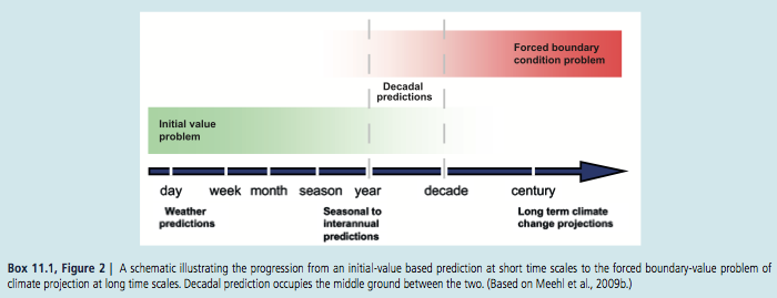
From IPCC AR5 Chapter 11

Figure 1

And in the introduction, chapter 1:

Climate in a narrow sense is usually defined as the average weather, or more rigorously, as the statistical description in terms of the mean and variability of relevant quantities over a period of time ranging from months to thousands or millions of years. The relevant quantities are most often surface variables such as temperature, precipitation and wind.

Classically the period for averaging these variables is 30 years, as defined by the World Meteorological Organization.

Climate in a wider sense also includes not just the mean conditions, but also the associated statistics (frequency, magnitude, persistence, trends, etc.), often combining parameters to describe phenomena such as droughts. Climate change refers to a change in the state of the climate that can be identified (e.g., by using statistical tests) by changes in the mean and/or the variability of its properties, and that persists for an extended period, typically decades or longer.

[Emphasis added].

Weather is an Initial Value Problem, Climate is a Boundary Value Problem

The idea is fundamental, the implementation is problematic.

As explained in Natural Variability and Chaos – Two – Lorenz 1963, there are two key points about a chaotic system:

1. With even a minute uncertainty in the initial starting condition, the predictability of future states is very limited
2. Over a long time period the statistics of the system are well-defined

(Being technical, the statistics are well-defined in a transitive system).

So in essence, we can’t predict the exact state of the future – from the current conditions – beyond a certain timescale which might be quite small. In fact, in current weather prediction this time period is about one week.

After a week we might as well say either “the weather on that day will be the same as now” or “the weather on that day will be the climatological average” – and either of these will be better than trying to predict the weather based on the initial state.

No one disagrees on this first point.

In current climate science and meteorology the term used is the skill of the forecast. Skill means, not how good is the forecast, but how much better is it than a naive approach like, “it’s July in New York City so the maximum air temperature today will be 28ºC”.

What happens in practice, as can be seen in the simple Lorenz system shown in Part Two, is a tiny uncertainty about the starting condition gets amplified. Two almost identical starting conditions will diverge rapidly – the “butterfly effect”. Eventually these two conditions are no more alike than one of the conditions and a time chosen at random from the future.

The wide divergence doesn’t mean that the future state can be anything. Here’s an example from the simple Lorenz system for three slightly different initial conditions:

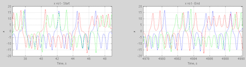
Figure 2

We can see that the three conditions that looked identical for the first 20 seconds (see figure 2 in Part Two) have diverged. The values are bounded but at any given time we can’t predict what the value will be.

On the second point – the statistics of the system, there is a tiny hiccup.

But first let’s review what is agreed upon. Climate is the statistics of weather. Weather is unpredictable more than a week ahead. Climate, as the statistics of weather, might be predictable. That is, just because weather is unpredictable, it doesn’t mean (or prove) that climate is also unpredictable.

This is what we find with simple chaotic systems.

So in the endeavor of climate modeling the best we can hope for is a probabilistic forecast. We have to run “a lot” of simulations and review the statistics of the parameter we are trying to measure.

To give a concrete example, we might determine from model simulations that the mean sea surface temperature in the western Pacific (between a certain latitude and longitude) in July has a mean of 29ºC with a standard deviation of 0.5ºC, while for a certain part of the north Atlantic it is 6ºC with a standard deviation of 3ºC. In the first case the spread of results tells us – if we are confident in our predictions – that we know the western Pacific SST quite accurately, but the north Atlantic SST has a lot of uncertainty. We can’t do anything about the model spread. In the end, the statistics are knowable (in theory), but the actual value on a given day or month or year are not.

Now onto the hiccup.

With “simple” chaotic systems that we can perfectly model (note 1) we don’t know in advance the timescale of “predictable statistics”. We have to run lots of simulations over long time periods until the statistics converge on the same result. If we have parameter uncertainty (see Ensemble Forecasting) this means we also have to run simulations over the spread of parameters.

Here’s my suggested alternative of the initial value vs boundary value problem:

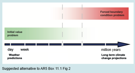
Figure 3

So one body made an ad hoc definition of climate as the 30-year average of weather.

If this definition is correct and accepted then “climate” is not a “boundary value problem” at all. Climate is an initial value problem and therefore a massive problem given our ability to forecast only one week ahead.

Suppose, equally reasonably, that the statistics of weather (=climate), given constant forcing (note 2), are predictable over a 10,000 year period.

In that case we can be confident that, with near perfect models, we have the ability to be confident about the averages, standard deviations, skews, etc of the temperature at various locations on the globe over a 10,000 year period.

Conclusion

The fact that chaotic systems exhibit certain behavior doesn’t mean that 30-year statistics of weather can be reliably predicted.

30-year statistics might be just as dependent on the initial state as the weather three weeks from today.

Articles in the Series

Natural Variability and Chaos – One – Introduction

Natural Variability and Chaos – Two – Lorenz 1963

Natural Variability and Chaos – Three – Attribution & Fingerprints

Natural Variability and Chaos – Four – The Thirty Year Myth

Natural Variability and Chaos – Five – Why Should Observations match Models?

Natural Variability and Chaos – Six – El Nino

Natural Variability and Chaos – Seven – Attribution & Fingerprints Or Shadows?

Natural Variability and Chaos – Eight – Abrupt Change

Notes

Note 1: The climate system is obviously imperfectly modeled by GCMs, and this will always be the case. The advantage of a simple model is we can state that the model is a perfect representation of the system – it is just a definition for convenience. It allows us to evaluate how slight changes in initial conditions or parameters affect our ability to predict the future.

The IPCC report also has continual reminders that the model is not reality, for example, chapter 11, p. 982:

For the remaining projections in this chapter the spread among the CMIP5 models is used as a simple, but crude, measure of uncertainty. The extent of agreement between the CMIP5 projections provides rough guidance about the likelihood of a particular outcome. But — as partly illustrated by the discussion above — it must be kept firmly in mind that the real world could fall outside of the range spanned by these particular models.

[Emphasis added].

Chapter 1, p.138:

Model spread is often used as a measure of climate response uncertainty, but such a measure is crude as it takes no account of factors such as model quality (Chapter 9) or model independence (e.g., Masson and Knutti, 2011; Pennell and Reichler, 2011), and not all variables of interest are adequately simulated by global climate models..

..Climate varies naturally on nearly all time and space scales, and quantifying precisely the nature of this variability is challenging, and is characterized by considerable uncertainty.

I haven’t yet been able to determine how these firmly noted and challenging uncertainties have been factored into the quantification of 95-100%, 99-100%, etc, in the various chapters of the IPCC report.

Note 2:  There are some complications with defining exactly what system is under review. For example, do we take the current solar output, current obliquity,precession and eccentricity as fixed? If so, then any statistics will be calculated for a condition that will anyway be changing. Alternatively, we can take these values as changing inputs in so far as we know the changes – which is true for obliquity, precession and eccentricity but not for solar output.

The details don’t really alter the main point of this article.

Read Full Post »

I’ve been somewhat sidetracked on this series, mostly by starting up a company and having no time, but also by the voluminous distractions of IPCC AR5. The subject of attribution could be a series by itself but as I started the series Natural Variability and Chaos it makes sense to weave it into that story.

In Part One and Part Two we had a look at chaotic systems and what that might mean for weather and climate. I was planning to develop those ideas a lot more before discussing attribution, but anyway..

AR5, Chapter 10: Attribution is 85 pages on the idea that the changes over the last 50 or 100 years in mean surface temperature – and also some other climate variables – can be attributed primarily to anthropogenic greenhouse gases.

The technical side of the discussion fascinated me, but has a large statistical component. I’m a rookie with statistics, and maybe because of this, I’m often suspicious about statistical arguments.

Digression on Statistics

The foundation of a lot of statistics is the idea of independent events. For example, spin a roulette wheel and you get a number between 0 and 36 and a color that is red, black – or if you’ve landed on a zero, neither.

The statistics are simple – each spin of the roulette wheel is an independent event – that is, it has no relationship with the last spin of the roulette wheel. So, looking ahead, what is the chance of getting 5 two times in a row? The answer (with a 0 only and no “00” as found in some roulette tables) is 1/37 x 1/37 = 0.073%.

However, after you have spun the roulette wheel and got a 5, what is the chance of a second 5? It’s now just 1/37 = 2.7%. The past has no impact on the future statistics. Most of real life doesn’t correspond particularly well to this idea, apart from playing games of chance like poker and so on.

I was in the gym the other day and although I try and drown it out with music from my iPhone, the Travesty (aka “the News”) was on some of the screens in the gym – with text of the “high points” on the screen aimed at people trying to drown out the annoying travestyreaders. There was a report that a new study had found that autism was caused by “Cause X” – I have blanked it out to avoid any unpleasant feeling for parents of autistic kids – or people planning on having kids who might worry about “Cause X”.

It did get me thinking – if you have let’s say 10,000 potential candidates for causing autism, and you set the bar at 95% probability of rejecting the hypothesis that a given potential cause is a factor, what is the outcome? Well, if there is a random spread of autism among the population with no actual cause (let’s say it is caused by a random genetic mutation with no link to any parental behavior, parental genetics or the environment) then you will expect to find about 500 “statistically significant” factors for autism simply by testing at the 95% level. That’s 500, when none of them are actually the real cause. It’s just chance. Plenty of fodder for pundits though.

That’s one problem with statistics – the answer you get unavoidably depends on your frame of reference.

The questions I have about attribution are unrelated to this specific point about statistics, but there are statistical arguments in the attribution field that seem fatally flawed. Luckily I’m a statistical novice so no doubt readers will set me straight.

On another unrelated point about statistical independence, only slightly more relevant to the question at hand, Pirtle, Meyer & Hamilton (2010) said:

In short, we note that GCMs are commonly treated as independent from one another, when in fact there are many reasons to believe otherwise. The assumption of independence leads to increased confidence in the ‘‘robustness’’ of model results when multiple models agree. But GCM independence has not been evaluated by model builders and others in the climate science community. Until now the climate science literature has given only passing attention to this problem, and the field has not developed systematic approaches for assessing model independence.

.. end of digression

Attribution History

In my efforts to understand Chapter 10 of AR5 I followed up on a lot of references and ended up winding my way back to Hegerl et al 1996.

Gabriele Hegerl is one of the lead authors of Chapter 10 of AR5, was one of the two coordinating lead authors of the Attribution chapter of AR4, and one of four lead authors on the relevant chapter of AR3 – and of course has a lot of papers published on this subject.

As is often the case, I find that to understand a subject you have to start with a focus on the earlier papers because the later work doesn’t make a whole lot of sense without this background.

This paper by Hegerl and her colleagues use the work of one of the co-authors, Klaus Hasselmann – his 1993 paper “Optimal fingerprints for detection of time dependent climate change”.

Fingerprints, by the way, seems like a marketing term. Fingerprints evokes the idea that you can readily demonstrate that John G. Doe of 137 Smith St, Smithsville was at least present at the crime scene and there is no possibility of confusing his fingerprints with John G. Dode who lives next door even though their mothers could barely tell them apart.

This kind of attribution is more in the realm of “was it the 6ft bald white guy or the 5’5″ black guy”?

Well, let’s set aside questions of marketing and look at the details.

Detecting GHG Climate Change with Optimal Fingerprint Methods in 1996

The essence of the method is to compare observations (measurements) with:

• model runs with GHG forcing
• model runs with “other anthropogenic” and natural forcings
• model runs with internal variability only

Then based on the fit you can distinguish one from the other. The statistical basis is covered in detail in Hasselmann 1993 and more briefly in this paper: Hegerl et al 1996 – both papers are linked below in the References.

At this point I make another digression.. as regular readers know I am fully convinced that the increases in CO2, CH4 and other GHGs over the past 100 years or more can be very well quantified into “radiative forcing” and am 100% in agreement with the IPCCs summary of the work of atmospheric physics over the last 50 years on this topic. That is, the increases in GHGs have led to something like a “radiative forcing” of 2.8 W/m² [corrected, thanks to niclewis].

And there isn’t any scientific basis for disputing this “pre-feedback” value. It’s simply the result of basic radiative transfer theory, well-established, and well-demonstrated in observations both in the lab and through the atmosphere. People confused about this topic are confused about science basics and comments to the contrary may be allowed or more likely will be capriciously removed due to the fact that there have been more than 50 posts on this topic (post your comments on those instead). See The “Greenhouse” Effect Explained in Simple Terms and On Uses of A 4 x 2: Arrhenius, The Last 15 years of Temperature History and Other Parodies.

Therefore, it’s “very likely” that the increases in GHGs over the last 100 years have contributed significantly to the temperature changes that we have seen.

To say otherwise – and still accept physics basics – means believing that the radiative forcing has been “mostly” cancelled out by feedbacks while internal variability has been amplified by feedbacks to cause a significant temperature change.

Yet this work on attribution seems to be fundamentally flawed.

Here was the conclusion:

We find that the latest observed 30-year trend pattern of near-surface temperature change can be distinguished from all estimates of natural climate variability with an estimated risk of less than 2.5% if the optimal fingerprint is applied.

With the caveats, that to me, eliminated the statistical basis of the previous statement:

The greatest uncertainty of our analysis is the estimate of the natural variability noise level..

..The shortcomings of the present estimates of natural climate variability cannot be readily overcome. However, the next generation of models should provide us with better simulations of natural variability. In the future, more observations and paleoclimatic information should yield more insight into natural variability, especially on longer timescales. This would enhance the credibility of the statistical test.

Earlier in the paper the authors said:

..However, it is generally believed that models reproduce the space-time statistics of natural variability on large space and long time scales (months to years) reasonably realistic. The verification of variability of CGMCs [coupled GCMs] on decadal to century timescales is relatively short, while paleoclimatic data are sparce and often of limited quality.

..We assume that the detection variable is Gaussian with zero mean, that is, that there is no long-term nonstationarity in the natural variability.

[Emphasis added].

The climate models used would be considered rudimentary by today’s standards. Three different coupled atmosphere-ocean GCMs were used. However, each of them required “flux corrections”.

This method was pretty much the standard until the post 2000 era. The climate models “drifted”, unless, in deity-like form, you topped up (or took out) heat and momentum from various grid boxes.

That is, the models themselves struggled (in 1996) to represent climate unless the climate modeler knew, and corrected for, the long term “drift” in the model.

Conclusion

In the next article we will look at more recent work in attribution and fingerprints and see whether the field has developed.

But in this article we see that the conclusion of an attribution study in 1996 was that there was only a “2.5% chance” that recent temperature changes could be attributed to natural variability. At the same time, the question of how accurate the models were in simulating natural variability was noted but never quantified. And the models were all “flux corrected”. This means that some aspects of the long term statistics of climate were considered to be known – in advance.

So I find it difficult to accept any statistical significance in the study at all.

If the finding instead was introduced with the caveat “assuming the accuracy of our estimates of long term natural variability of climate is correct..” then I would probably be quite happy with the finding. And that question is the key.

The question should be:

What is the likelihood that climate models accurately represent the long-term statistics of natural variability?

• Virtually certain
• Very likely
• Likely
• About as likely as not
• Unlikely
• Very unlikely
• Exceptionally unlikely

So far I am yet to run across a study that poses this question.

Articles in the Series

Natural Variability and Chaos – One – Introduction

Natural Variability and Chaos – Two – Lorenz 1963

Natural Variability and Chaos – Three – Attribution & Fingerprints

Natural Variability and Chaos – Four – The Thirty Year Myth

Natural Variability and Chaos – Five – Why Should Observations match Models?

Natural Variability and Chaos – Six – El Nino

Natural Variability and Chaos – Seven – Attribution & Fingerprints Or Shadows?

Natural Variability and Chaos – Eight – Abrupt Change

References

Bindoff, N.L., et al, 2013: Detection and Attribution of Climate Change: from Global to Regional. In: Climate Change 2013: The Physical Science Basis. Contribution of Working Group I to the Fifth Assessment Report of the Intergovernmental Panel on Climate Change

Detecting greenhouse gas induced climate change with an optimal fingerprint method, Hegerl, von Storch, Hasselmann, Santer, Cubasch & Jones, Journal of Climate (1996)

What does it mean when climate models agree? A case for assessing independence among general circulation models, Zachary Pirtle, Ryan Meyer & Andrew Hamilton, Environ. Sci. Policy (2010)

Optimal fingerprints for detection of time dependent climate change, Klaus Hasselmann, Journal of Climate (1993)

Read Full Post »