In Part Seven we had a look at a 2008 paper by Gettelman & Fu which assessed models vs measurements for water vapor in the upper troposphere.
In this article we will look at a 2010 paper by Chung, Yeomans & Soden. This paper studies outgoing longwave radiation (OLR) vs temperature change, for clear skies only, in three ways (and comparing models and measurements):
- by region
- by season
- year to year
Why is this important and what is the approach all about?
Let’s suppose that the surface temperature increases for some reason. What happens to the total annual radiation emitted by the climate system? We expect it to increase. The hotter objects are the more they radiate.
If there is no positive feedback in the climate system then for a uniform global 1K (=1ºC) increase in surface & atmospheric temperature we expect the OLR to increase by 3.6 W/m². This is often called, by convention only, the “Planck feedback”. It refers to the fact that an increased surface temperature, and increased atmospheric temperature, will radiate more – and the “no feedback value” is 3.6 W/m² per 1K rise in temperature.
To explain a little further for newcomers.. with the concept of “no positive feedback” an initial 1K surface temperature rise – from any given cause – will stay at 1K. But if there is positive feedback in the climate system, an initial 1K surface temperature rise will result in a final temperature higher than 1K.
If the OLR increases by less than 3.6 W/m² the final temperature will end up higher than 1K – positive feedback. If the OLR increases by more than 3.6 W/m² the final temperature will end up lower than 1K – negative feedback.
Base Case
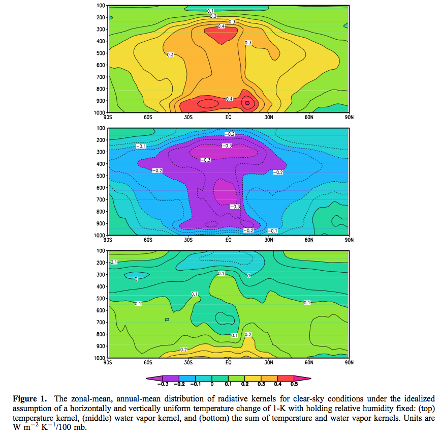
At the start of their paper they show the calculated clear-sky OLR change as the result of an ideal case. This is the change in OLR as a result of the surface and atmosphere increasing uniformly by 1K:
- first, from the temperature change alone
- second, from the change in water vapor as a result of this temperature change, assuming relative humidity stays constant
- finally, from the first and second combined
From Chung et al (2010)
Figure 1 – Click to expand
The graphs show the breakdown by pressure (=height) and latitude. 1000mbar is the surface and 200mbar is approximately the tropopause, the place where convection stops.
The sum of the first graph (note 1) is the “no feedback” response and equals 3.6 W/m². The sum of the second graph is the “feedback from water vapor” and equals -1.6 W/m². The combined result in the third graph equals 2.0 W/m². The second and third graphs are the result if relative humidity is constant.
We can also see that the tropics is where most of the changes take place.
They say:
One striking feature of the fixed-RH kernel is the small values in the tropical upper troposphere, where the positive OLR response to a temperature increase is offset by negative responses to the corresponding vapor increase. Thus under a constant RH- warming scenario, the tropical upper troposphere is in a runaway greenhouse state – the stabilizing effect of atmospheric warming is neutralized by the increased absorption from water vapor. Of course, the tropical upper troposphere is not isolated but is closely tied to the lower tropical troposphere where the combined temperature-water vapor responses are safely stabilizing.
To understand the first part of their statement, if temperatures increase and overall OLR does not increase at all then there is nothing to stop temperatures increasing. Of course, in practice, the “close to zero” increase in OLR for the tropical upper troposphere under a temperature rise can’t lead to any kind of runaway temperature increase. This is because there is a relationship between the temperatures in the upper troposphere and the lower- & mid- troposphere.
Relative Humidity Stays Constant?
Back in 1967, Manabe & Wetherald published their seminal paper which showed the result of increases in CO2 under two cases – with absolute humidity constant and with relative humidity constant:
Generally speaking, the sensitivity of the surface equilibrium temperature upon the change of various factors such as solar constant, cloudiness, surface albedo, and CO2 content are almost twice as much for the atmosphere with a given distribution of relative humidity as for that with a given distribution of absolute humidity..
..Doubling the existing CO2 content of the atmosphere has the effect of increasing the surface temperature by about 2.3ºC for the atmosphere with the realistic distribution of relative humidity and by about 1.3ºC for that with the realistic distribution of absolute humidity.
They explain important thinking about this topic:
Figure 1 shows the distribution of relative humidity as a function of latitude and height for summer and winter. According to this figure, the zonal mean distributions of relative humidity closely resemble one another, whereas those of absolute humidity do not. These data suggest that, given sufficient time, the atmosphere tends to restore a certain climatological distribution of relative humidity responding to the change of temperature.
It doesn’t mean that anyone should assume that relative humidity stays constant under a warmer world. It’s just likely to be a more realistic starting point than assuming that absolute humidity stays constant.
I only point this out for readers to understand that this idea is something that has seemed reasonable for almost 50 years. Of course, we have to question this “reasonable” assumption. How relative humidity changes as the climate warms or cools is a key factor in determining the water feedback and, therefore, it has had a lot of attention.
Results From the Paper
The observed rates of radiative damping from regional, seasonal, and interannual variations are substantially smaller than the rate of Planck radiative damping (3.6W/m²), yet slightly larger than that anticipated from a uniform warming, constant-RH response (2.0 W/m²).
The three comparison regressions can be seen, with ERBE data on the left and model results on the right:
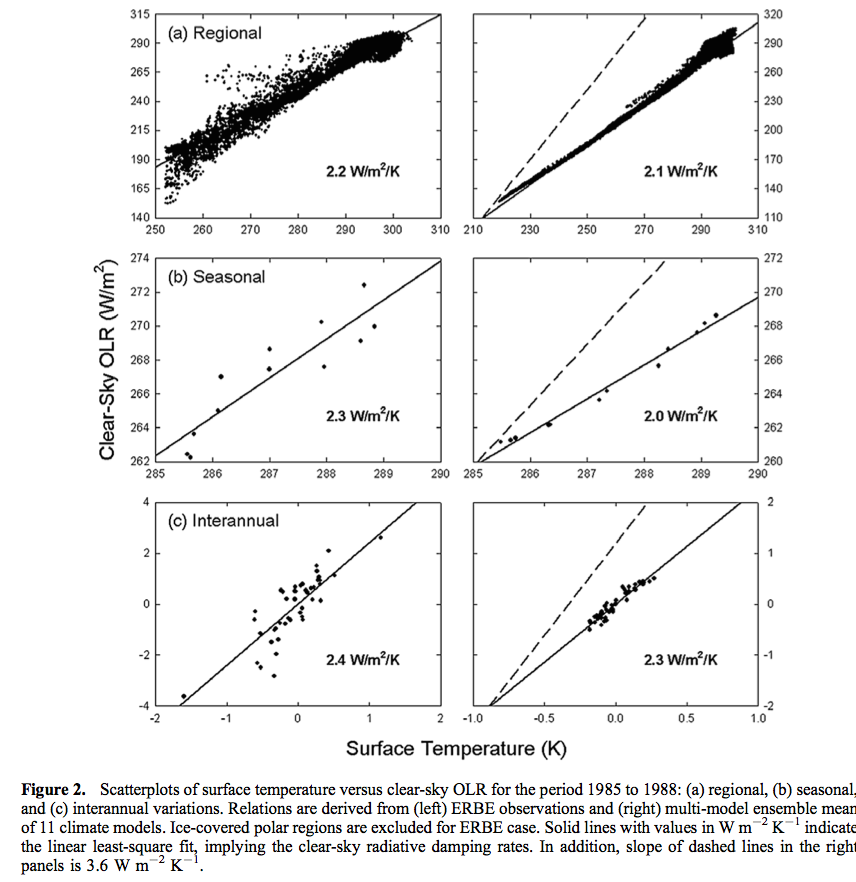
From Chung et al (2010)
Figure 2 – Click to expand
In the next figure, the differences between the models can be seen, and compared with ERBE and CERES results. The red “Planck” line is the no-feedback line, showing that (for these sets of results) models and experimental data show a positive feedback (when looking at clear sky OLR).
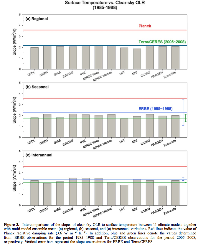
From Chung et al (2010)
Figure 3 – Click to expand
Conclusion
At the least, we can see that climate models and measured values are quite close, when the results are aggregated. Both the model and the measured results are a long way from neutral feedback (the dashed slope in figure 2 and the red line in figure 3), instead they show positive feedback, quite close to what we would expect from constant relative humidity. The results indicate that relative humidity declines a little in the warmer case. The results also indicate that the models calculate a little more positive feedback than the real world measurements under these cases.
What does this mean for feedback from warming from increased GHGs? It’s the important question. We could say that the results tell us nothing, because how the world warms from increasing CO2 (and other GHGs) will change climate patterns and so seasonal, regional and year to year changes in periods from 1985-1988 and 2005-2008 are not particularly useful.
We could say that the results tell us that water vapor feedback is demonstrated to be a positive feedback, and matches quite closely the results of models. Or we could say that without cloudy sky data the results aren’t very interesting.
At the very least we can see that for current climate conditions under clear skies the change in OLR as temperature changes indicates an overall positive feedback, quite close to constant relative humidity results and quite close to what models calculate.
The ERBE results include the effect of a large El Nino and I do question whether year to year changes (graph c in figs 2 & 3) under El Nino to La Nino changes can be considered to represent how the climate might warm with more CO2. If we consider how the weather patterns shift during El-Nino to La Nina it has long been clear that there are positive feedbacks, but also the weather patterns end up back to normal (the cycle ends). I welcome knowledgeable readers explaining why El Nino feedback patters are relevant to future climate shifts, perhaps this will help me to clarify my thinking, or correct my misconceptions.
However, the CERES results from 2005-2008 don’t include the effect of a large El Nino and they show an overall slightly more positive feedback.
I asked Brian Soden a few question about this paper and he was kind enough to respond:
Q. Given the much better quality data since CERES and AIRS, why is ERBE data the focus?
A. At the time, the ERBE data was the only measurement that covered a large ENSO cycle (87/88 El Nino event followed by 88/89 La Nina)
Q. Why not include cloudy skies as well in this review? Collecting surface temperature data is more challenging of course because it needs a different data source. Is there a comparable study that you know of for cloudy skies?
A. The response of clouds to surface temperature changes is more complicated. We wanted to start with something relatively simple; i.e., water vapor. Andrew Dessler at Texas AM has a paper that came out a few years back that looks at total-sky fluxes and thus includes the effects on clouds.
Q. Do you know of any studies which have done similar work with what must now be over 10 years of CERES/AIRS.
A. Not off-hand. But it would be useful to do.
Articles in the Series
Part One – introducing some ideas from Ramanathan from ERBE 1985 – 1989 results
Part One – Responses – answering some questions about Part One
Part Two – some introductory ideas about water vapor including measurements
Part Three – effects of water vapor at different heights (non-linearity issues), problems of the 3d motion of air in the water vapor problem and some calculations over a few decades
Part Four – discussion and results of a paper by Dessler et al using the latest AIRS and CERES data to calculate current atmospheric and water vapor feedback vs height and surface temperature
Part Five – Back of the envelope calcs from Pierrehumbert – focusing on a 1995 paper by Pierrehumbert to show some basics about circulation within the tropics and how the drier subsiding regions of the circulation contribute to cooling the tropics
Part Six – Nonlinearity and Dry Atmospheres – demonstrating that different distributions of water vapor yet with the same mean can result in different radiation to space, and how this is important for drier regions like the sub-tropics
Part Seven – Upper Tropospheric Models & Measurement – recent measurements from AIRS showing upper tropospheric water vapor increases with surface temperature
Part Eight – Clear Sky Comparison of Models with ERBE and CERES – a paper from Chung et al (2010) showing clear sky OLR vs temperature vs models for a number of cases
Part Nine – Data I – Ts vs OLR – data from CERES on OLR compared with surface temperature from NCAR – and what we determine
Part Ten – Data II – Ts vs OLR – more on the data
References
An assessment of climate feedback processes using satellite observations of clear-sky OLR, Eui-Seok Chung, David Yeomans, & Brian J. Soden, GRL (2010) – free paper
Thermal equilibrium of the atmosphere with a given distribution of relative humidity, Manabe & Wetherald, Journal of the Atmospheric Sciences (1967) – free paper
Notes
Note 1: The values are per 100 mbar “slice” of the atmosphere. So if we want to calculate the total change we need to sum the values in each vertical slice, and of course, because they vary through latitude we need to average the values (area-weighted) across all latitudes.


