The Science of Doom

In Part Two we covered quite a bit of ground. At the end we looked at the first calculation of heating rates. The values calculated were a little different in magnitude from results in a textbook, but the model was still in a rudimentary phase.

After numerous improvements – outlined in Part Five – The Code, I got around to adding some “standard atmospheres” so we can see some comparisons and at least see where this model departs from other more accurate models.

First, what are heating rates? Within the context of this model we are currently thinking about the longwave radiative heating rates, which really means this:

If the only part of climate physics that was actually working was “longwave radiation” (terrestrial radiation) then how fast would different parts of the atmosphere heat up or cool down?

As we will see this mechanism (terrestrial radiation) mostly results in a net cooling for each part of the atmosphere.

The atmosphere also absorbs solar radiation – not shown in these graphs – which acts in the opposite direction and provides a heating.

Lastly, the sun warms the surface and convection transfers heat much more efficiently from the surface to the lower atmosphere – and this makes up the balance.

So, with longwave heating (cooling) curves, we are consider one mechanism of how heat is transferred.

Second, what is “longwave radiation”? This is a conventional description of the radiation emitted by the climate system, specifically the fact that its wavelength is almost all above 4 μm. The other significant radiation component in the climate system is “shortwave radiation”, which by convention means radiation below 4 μm. See The Sun and Max Planck Agree – Part Two for more.

Third, what is a “standard atmosphere”? It’s just a kind of average, useful for inter-comparisons, and for evaluation of various climate mechanisms around ideal cases. In this case, I used the AFGL (air force geophysics lab) models which are also used in the LBLTRM (line by line radiative transfer model).

Here is a graph for tropical conditions of heating rate vs height – and with a breakdown between the rates caused by water vapor, CO2 and O3:

Figure 1

Notice that the heating rate is mostly negative, so the atmosphere is cooling via radiation – which means for this atmospheric profile water vapor, CO2 and ozone have a net effect of emitting more terrestrial radiation out than they absorb via these gases.

Here is a textbook comparison:

Figure 2

And a set of graphs detailing the tropical condition for temperature, pressure, density and GHG concentrations:

Figure 3 – Click to enlarge

Now some comparisons of the overall heating rates for 3 different profiles:

Figure 4

Here is a textbook comparison:

Figure 5

So we can see that the MATLAB model created here from first principles and using the HITRAN database of absorption and emission lines is quite close to other calculated standards.

In fact, the differences are small except in the mid-stratosphere and we may find that this is due to slight differences in the model atmosphere used, or as a result of not using the Voigt profile (this is an important but technical area of atmospheric radiation – line shapes and how they change with pressure and temperature in the atmosphere – see for example Part Eight – CO2 Under Pressure).

Pekka Pirilä has been running this MATLAB model as well, has helped with numerous improvements and has just implemented the Voigt profile so we will shortly find out if the line shape is a contributor to any differences.

For reference, here are the profiles of the other two conditions shown in figure 4: Midlatitude summer & Subarctic summer:

Figure 6 – Click to enlarge

Figure 7 – Click to enlarge

Related Articles

Part One – some background and basics

Part Two – some early results from a model with absorption and emission from basic physics and the HITRAN database

Part Three – Average Height of Emission – the complex subject of where the TOA radiation originated from, what is the “Average Height of Emission” and other questions

Part Four – Water Vapor – results of surface (downward) radiation and upward radiation at TOA as water vapor is changed

Part Five – The Code – code can be downloaded, includes some notes on each release

Part Six – Technical on Line Shapes – absorption lines get thineer as we move up through the atmosphere..

Part Seven – CO2 increases – changes to TOA in flux and spectrum as CO2 concentration is increased

Part Eight – CO2 Under Pressure – how the line width reduces (as we go up through the atmosphere) and what impact that has on CO2 increases

Part Nine – Reaching Equilibrium – when we start from some arbitrary point, how the climate model brings us back to equilibrium (for that case), and how the energy moves through the system

Part Ten – “Back Radiation” – calculations and expectations for surface radiation as CO2 is increased

Part Eleven – Stratospheric Cooling – why the stratosphere is expected to cool as CO2 increases

Part Thirteen – Surface Emissivity – what happens when the earth’s surface is not a black body – useful to understand seeing as it isn’t..

References

AFGL atmospheric constituent profiles (0.120 km), by GP Anderson et al (1986)

A First Course in Atmospheric Radiation, Grant Petty, Sundog Publishing (2006)

The data used to create these graphs comes from the HITRAN database.

The HITRAN 2008 molecular spectroscopic database, by L.S. Rothman et al, Journal of Quantitative Spectroscopy & Radiative Transfer (2009)

The HITRAN 2004 molecular spectroscopic database, by L.S. Rothman et al., Journal of Quantitative Spectroscopy & Radiative Transfer (2005)

Read Full Post »

Understanding atmospheric radiation is not so simple. But now we have a line by line model of absorption and emission of radiation in the atmosphere we can do some “experiments”. See Part Two and Part Five – The Code.

Many people think that models are some kind of sham and climate scientists should be out there doing real experiments. Well, models aren’t a sham and climate scientist are out there doing lots of experiments. Various articles on Science of Doom have outlined some of the very detailed experiments that have been done by atmospheric physicists, aka climate scientists.

When you want to understand why some aspect of a climate mechanism works the way it does, or what happens if something changes then usually you have to resort to a mathematical model of that part of the climate.

You can’t suddenly increase the amount of a major GHG across the planet, or slow down the planetary rotation to ½ its normal speed. Well, not without a sizable investment, a health and safety risk, possible inconvenience to a lot of people and, at some stage, awkward government investigations.

You can’t stop the atmosphere emitting radiation or test a stratosphere that gets cooler with height. But you can attempt to model it.

Mathematical models all have their limitations. We have to understand what the model can tell us and what it can’t tell us. We have to understand what presuppositions are built into the model and what can change in real life that is not being modeled in the maths. It’s all about context.

(Well-designed) models are not correct and are not incorrect. They are informative if we understand their limitations and capabilities.

In contrast to mathematical models built around the physics of climate mechanisms, many people commenting in the blog world (or even writing blogs) have a vague mental model of how climate works. This of course is way way ahead of a climate model built on physics. It has the advantage of not being written down in equations so that no one can challenge it and seemingly plausible hand-waving argument 1 can be traded against hand-waving argument 2. Unfortunately, on this blog we don’t have the luxury of those resources and – where experiments are not available or not possible – we will have to evaluate the results of mathematical models built on physics and observations.

All the above is not an endorsement of what GCMs tell us. And not an indictment. Hopefully no one reading the above paragraphs came to either conclusion.

When I first built the line by line model it had more limitations than today. One early problem was the stratosphere. In real life the temperature of the stratosphere increases with height. In the model the temperature decreased with height.

This was expected. O2 and O3 absorb solar radiation (primarily ultraviolet) and warm mainly the middle layers of the stratosphere. But the model didn’t have this physics. The model, at this stage, primarily modeled the absorption and emission of terrestrial (aka ‘longwave’) radiation by the atmosphere.

So, after a few versions a very crude model of solar absorption was added. Unfortunately, this solar absorption model still did not create a stratosphere that increased with temperature. This was quite disappointing.

Then commenter Uli pointed out that the model had too much stratospheric water vapor and I added a new parameter to the model which allowed stratospheric water vapor to be set differently from the free troposphere. (So far I’ve been using a realistic level of 6ppmv).

The result was happily that the stratosphere, left to its own (model) devices, started increasing with temperature. The starting point is simply a temperature profile dictated to the model, and the finish point is how the physics ends up calculating the final temperature profile:

Figure 1 – A warmer stratosphere and a happier climate model

At the same time, I’ve been updating the model so that it can run to some kind of equilbrium and then various GHGs can be changed.

This was to calculate “radiative forcing” under various scenarios, and specifically I wanted to show how energy moved around in the climate system after a “bump” in something like CO2. This is something that many many people can’t get right in their heads. One of the objectives of the model is to show bit by bit how the increased CO2 causes a reduction in net outgoing radiation, and how that in turn pushes up the atmospheric and surface temperature.

On this journey, once the model stratosphere was behaving a little like its real-life big brother it occurred to me that maybe we could answer the question of why the stratosphere was expected to cool with increased CO2.

See Stratospheric Cooling for some background.

Previously I have worked under the assumption that there are lots of competing “terms” in the energy balance equation for how the stratosphere responds to more CO2 and so simple conceptual models are not going to help.

Now the Science of Doom Climate Model (SoDCM) comes to the rescue.

In fact, while I was waiting for lots of simulations to finish on the PC I was reading again the fascinating Radiative Forcing and Climate Response, by Hansen, Sato & Ruedy, JGR (1997) – free paper – and in a groundhog day experience realized I didn’t understand their flux graphs resulting from various GCM simulations. So the SoDCM allowed me to solve my own conceptual problems.

Maybe.

Let’s take a look at stratospheric cooling.

Understanding Flux Curves

In this simulation:

• CO2 at 280 ppm
• no ozone, CH4 or NO2 for longwave absorption
• boundary layer humidity at 80%
• free tropospheric humidity at 40%
• stratospheric water vapor at 6 ppmv
• tropopause at 200 hPa
• top of atmosphere (TOA) at 1 hPa
• solar radiation at 242 W/m² with some absorbed in the stratosphere and troposphere as shown in figure 1 of Part Nine – Reaching Equilibrium

The surface temperature reached equilibrium at 281K and the tropopause was at 11 km:

Figure 2

The equilibrium was reached by running the model for 500 (model) days, with timesteps of 2 hours. The ocean depth was only 5 meters simply to allow the model to get to equilibrium quicker (note 1).

Then at 500 days the CO2 concentration was doubled to 560 ppm and we capture a number of different values from the timestep before the increase and the timestep after the increase.

Let’s take a look at the up and down fluxes through the atmosphere. See also figure 6 of Part Two. In this case we can see pre- and post-2xCO2, but let’s first just try and understand what these flux vs height graphs actually mean:

Figure 3 – Understanding the Basics

If flux just stays constant (vertical line) through a section of the atmosphere what does it mean?

It means there is no net absorption. It could mean that the atmosphere is transparent to that radiation. It could mean that the atmosphere emits exactly the same amount that it absorbs. Or some of both. Either way, no change = no net radiation absorbed.

Take a look in figure 3 at the (pre-CO2 doubling) upward flux above 10km (in the stratosphere). About 237 W/m² enters the bottom of the stratosphere and about 242 W/m² leaves the top of atmosphere. So the stratosphere is 5 W/m² worse off and from the first law of thermodynamics this either cools the stratosphere or something else is supplying this energy.

Now take a look at the (pre-CO2) downward flux in the stratosphere. At the top of atmosphere there is no downward longwave radiation because there is no source of this radiation outside of the atmosphere. So downward flux = 0 at TOA.

At the bottom of the stratosphere, about 27 W/m² is leaving. So zero is entering and 27 W/m² is leaving – this means that the stratosphere is worse off by 27 W/m².

If we add up the upward and downward longwave fluxes through the stratosphere we find that there is a net loss of about 32 W/m². This means that if the stratosphere is in equilibrium some other source must be supplying 32 W/m².

In this case it is the solar absorption of radiation.

If we were considering the troposphere it would most likely be convection from the surface or lower atmosphere that would be balancing any net radiation loss from higher up in the troposphere.

So, to recap:

• think about the direction radiation is travelling in:
  • if it is reducing in the direction it is travelling then energy is absorbed into that section of the atmosphere
  • if it is increasing in the direction it is travelling then energy is being lost from that section of the atmosphere
• if plots of flux against height are vertical that means there is no change in energy in that region
• if flux vs height is constant (vertical) then it either means
  • the atmosphere is transparent to that radiation, OR
  • the atmosphere is isothermal in that region (emission is balanced by absorption)

Take another look at figure 3 below 10km:

1. The upward radiation is reducing with height – energy is absorbed by each level of the atmosphere. This is a net heating.
2. The downward radiation is increasing – energy is lost from each level of the atmosphere. This is a net cooling.
3. The slope of the curves is not equal. This is because energy is transferred via convection in the troposphere.

Understanding these concepts is essential to understanding radiation in the atmosphere.

Upward Flux from Changes in CO2

Let’s take a closer look at the upward and downward changes due to doubling CO2. So the “pre” curve is the atmosphere in a nice equilibrium condition. And the “post” curve is immediately after CO2 has been doubled, long before any equilibrium has been reached.

Let’s zoom in on the upward fluxes in the stratosphere pre- and immediately post-CO2 doubling:

Figure 4

Even though the curves are roughly parallel from 10km through to 30km you should be able to see that there is a larger gradient on the post-2xCO2 curve. So pre-CO2 increase, the stratosphere loses a net upward of about 5 W/m², and after CO2 increase the stratosphere loses a net upward of about 6 W/m².

This means more CO2 increases the cooling of the stratosphere when we consider the upward flux. So now the question is, WHY?

If we want to understand the answer, the most useful ingredient is to look at the spectral characteristics of pre- and post. Here we take the radiation leaving at TOA and subtract the radiation entering at the tropopause. So we are considering the net energy lost (why lost? because this calculation is energy out – energy in), and as a function of wavenumber.

Here is the spectral graph of energy lost by the stratosphere due to upwards radiation, before the CO2 increase:

Figure 5

The post-CO2 doubling looks very similar so here is a comparison graph, with a slight smoothing (moving average window) just to allow us to see a little more clearly the main differences:

Figure 6

So we see that in the case of post-2xCO2, the energy lost is a little higher, and it is in the wavenumber region where CO2 emits strongly. CO2’s peak absorption/emission is at 667 cm^-1 (15 μm).

Just to confirm, here is the difference – post-2xCO2 minus pre-2xCO2 and not smoothed:

Figure 7

We can see that the main regions of CO2 absorption and emission are the reason. And we note that the temperature of the stratosphere is increasing with height.

So the reason is clear – due to principles outlined earlier in Part Two. Because the stratospheric temperature increases with height, the net emission (i.e., emission less absorption) of radiation, as we go up through the stratosphere will be a progressively higher value. And once we increase the amount of CO2, this net emission will increase even further.

This is what we see in the spectral intensity – the net change in stratospheric emission [(out-in)_2xCO2 – (out-in)_1xCO2] increases due to the emission in the main CO2 bands.

Downward Flux from Changes in CO2

Here is what we see when we zoom in on the downward flux in the stratosphere:

Figure 8

Of course, as already mentioned, the downward longwave flux at TOA must be zero.

This time it is conceptually easier to understand the change from more CO2. There’s one little fly in the understanding ointment, but let’s come to that later.

So when we think about the cooling of the stratosphere from downward flux it’s quite easy. Coming in at the top is zero. Coming out of the bottom (pre-CO2 increase) is about 27 W/m². Coming out of the bottom (post-2xCO2) is about 30 W/m². So increasing CO2 causes a cooling of about 3 W/m² due to changes in downward flux.

Here is the spectral flux (unsmoothed) downward out of the bottom of the tropopause, pre- and post-2xCO2:

Figure 9

And as with figure 7, below is the difference in downward intensity as a result of 2xCO2. This is post less pre, so the positive value overall means a cooling – as we saw in the total flux change in figure 8.

The cause is still due to the CO2 band but the specifics are a little different from the upward change. Here the center of the CO2 band has zero effect. But the “wings” of the CO2 band – around 600 cm^-1 and 700 cm^-1 are the places causing the effect:

Figure 10

The temperature is reducing as we go downwards so the emission from the center of the CO2 band cannot be increasing as we go downward. If we look back at figure 7 for the upward direction, the temperature is increasing upward so the emission from the center of the CO2 band must be increasing.

And the conceptual fly in the ointment alluded to earlier – this one can be confusing (or simple..) – if the starting flux at TOA is zero and the temperature decreases downward surely the downward flux only gets less? Less than zero? Instead, think of the whole stratosphere as a body. It must emit radiation due to its temperature and emissivity. It can’t absorb any radiation from above (because there is none), so it must emit some downward radiation. As its emissivity increases with more GHGs it must emit more radiation into the troposphere. It’s simple really.

Let’s now finalize this story by considering the net change in flux with height due to CO2 increases. Here if “net” is increasing with height it means absorption or heating. And if “net” is reducing with height it means emission or cooling. See note 2 where the details are explained.

So the blue line (upward flux) decreasing from the tropopause up to TOA means that the change in flux is cooling the stratosphere. And likewise for the green line (downward flux). This is just the results already shown as spectral changes now shown as flux changes:

Figure 11

Net Effect

If we combine figure 11 for the total net effect of doubling CO2:

Figure 12

From the tropopause at 11km through to TOA we can see that the combined change in flux due to CO2 doubling causes a cooling of the stratosphere. (And from the surface up to the tropopause we see a heating of the troposphere).

By comparison, here is an extract from Hansen et al (1997):

Figure 13

The highlighted instantaneous graph is the one for comparison with figure 12.

This is the case before the stratosphere has relaxed into equilibrium. Note that the “adjusted” graph – stratospheric equilibrium – has a vertical line for ΔF vs height, which simply means that the stratosphere is, in that case, in radiative equilibrium.

Notice as well that the magnitude of my graph is a lot higher. There may be a lot of reasons for that, including that fact that mine is one specific case rather than some climatic mean, and also that the absorption of solar radiation in my model has been treated very crudely. (Lots of other factors include missing GHGs like CH4, N2O, etc).

Reasons

So we have seen that the net emission of radiation by CO2 bands is what causes the cooling from upward radiation and the cooling from downward radiation when CO2 is increased.

For further insight, I amended the model so that on the timestep before and just after equilibrium the stratosphere was:

A) snapped back to an isothermal case, with the temperature set at the tropopause temperature just calculated

B) forced into a cooling at 4 K/km (c.f. the troposphere with a lapse rate of 6.5 K/km)

Case A, temperature profile just before and after equilibrium:

Figure 14

And the comparison to figure 11:

Figure 15

We can see that the downward flux change is similar to figure 11, but the upward flux is different. It is fairly constant through the stratosphere. This is not surprising. The flux from below is either transmitted straight through, or is absorbed and re-emitted at the same temperature. So no change to upward flux.

But the downward flux only results from the emission from the stratosphere (nothing transmitted through from above). As CO2 is increased the emissivity of the atmosphere increases and so emission of radiation from the stratosphere increases. The fact that the stratospheric temperature is isothermal has a small effect as can be seen by comparing the green curve on figures 15 & 11. But it isn’t very significant.

Now let’s consider case B. First the temperature profile:

Figure 16

Now the net flux graph:

Figure 17

Here we see that the effect of increased CO2 on the upward flux is now a heating in the stratosphere. And the net change in downward flux still has a cooling effect.

Figure 18

Here we see that for a stratosphere where temperature reduces with altitude, doubling CO2 would not have a noticeable effect on the stratospheric temperature. Depending on the temperature profile (and other factors) there might be a slight cooling or a slight heating.

Conclusion

This is a subject where it’s easy to confuse readers – along with the article writer. Possibly no one that was unclear before made it the whole way and said “ok, got it”.

Hopefully, if you only made it only part of the way through, you now have a better grasp of some of the principles.

The reasons behind stratospheric cooling due to increased GHGs have been difficult to explain even for very knowledgeable atmospheric physicists (e.g., one of many).

I think I can explain stratospheric cooling under increasing CO2. I think I can see that other factors like the exact temperature profile of the stratosphere on any given day/month and the water vapor profile (not shown in this article) will also affect the change in stratospheric temperature from increasing CO2.

If the bewildering complexity of up/down, in-out, net of in-out, net of in-out for 2xCO2-original CO2 has left you baffled please feel free to ask questions. This is not an easy topic. I was baffled. I have 4 pages of notes with little graphs and have rewritten the equations in note 2 at least 5 times to try and get the meaning clear – and am still expecting someone to point out a sign error.

Related Articles

Part One – some background and basics

Part Two – some early results from a model with absorption and emission from basic physics and the HITRAN database

Part Three – Average Height of Emission – the complex subject of where the TOA radiation originated from, what is the “Average Height of Emission” and other questions

Part Four – Water Vapor – results of surface (downward) radiation and upward radiation at TOA as water vapor is changed

Part Five – The Code – code can be downloaded, includes some notes on each release

Part Six – Technical on Line Shapes – absorption lines get thineer as we move up through the atmosphere..

Part Seven – CO2 increases – changes to TOA in flux and spectrum as CO2 concentration is increased

Part Eight – CO2 Under Pressure – how the line width reduces (as we go up through the atmosphere) and what impact that has on CO2 increases

Part Nine – Reaching Equilibrium – when we start from some arbitrary point, how the climate model brings us back to equilibrium (for that case), and how the energy moves through the system

Part Ten – “Back Radiation” – calculations and expectations for surface radiation as CO2 is increased

Part Twelve – Heating Rates – heating rate (‘C/day) for various levels in the atmosphere – especially useful for comparisons with other models.

References

The data used to create these graphs comes from the HITRAN database.

The HITRAN 2008 molecular spectroscopic database, by L.S. Rothman et al, Journal of Quantitative Spectroscopy & Radiative Transfer (2009)

The HITRAN 2004 molecular spectroscopic database, by L.S. Rothman et al., Journal of Quantitative Spectroscopy & Radiative Transfer (2005)

Radiative Forcing and Climate Response, by Hansen, Sato & Ruedy, JGR (1997) – free paper

Notes

Note 1: The relative heat capacity of the ocean vs the atmosphere has a huge impact on the climate dynamics. But in this simulation we were interested in reaching an equilibrium for a given CO2 concentration & solar absorption – and then seeing what happened to radiative balance immediately after a bump in CO2 concentration.

For this requirement it isn’t so important to have the right ocean depth needed for decent dynamic modeling.

Note 2: The treatment of upward and downward flux can get bewildering. The easiest approach is to just consider the change in flux in the direction in which it is travelling. But because upward and downward are in opposite directions, F↑ is in the direction of z, and F↓ is in the opposite direction to z, so heating and cooling are in opposite directions.

Due to changing GHGs:

If F↑(z)_2xCO2 – F↑(z) < 0 => Heating below height z (less flux escaping);

F↑(z)_2xCO2 – F↑(z) > 0  => Cooling below height z

If F↓(z)_2xCO2 – F↓(z) < 0 => Cooling below height z (less flux entering);

F↓(z)_2xCO2 – F↓(z) > 0  => Heating below height z

So for example for figure 11 – the net upward = F↑(z) – F↑(z)_2xCO2 & net downward = F↓(z)_2xCO2 – F↓(z)

Flux “divergence”

dF↑(z)/dz < 0  => Heating of that part of the atmosphere (upward flux is reducing due to being absorbed)

dF↓(z)/dz < 0  => Cooling of that part of the atmosphere (downward flux is increasing as we go down due to more being emitted, or rewritten is very strange English to match the equation: downward flux is decreasing in the upward direction)

Read Full Post »

We have mostly looked at the upward spectra at the top of atmosphere (TOA) as various conditions are changed. There’s a good reason for this focus – the outgoing longwave radiation (OLR) determines how much the climate system cools to space.

Over a given timescale this either matches absorbed solar radiation or the planet is heating or cooling. So it is changes in OLR (or absorbed solar) that really affect the heat balance in the climate.

By comparison, the trend in downward longwave radiation (DLR) at the surface is more a result of overall planetary heating and cooling. But of course, the climate is a lot more complex than indicated by that last statement.

Let’s take a look. Note that Part Four – Water Vapor already has some graphs of how the DLR or “back radiation” changes with water vapor concentration.

Here is the DLR for 4 different surface temperatures. In each case there is a lapse rate of 6.5 K/km, the boundary layer humidity (BLH) = 100%, the free tropospheric humidity (FTH) = 40% and there were 10 atmospheric layers in the model with a top of atmosphere at 50 hPa. More about the model in Part Two and Part Five – The Code.

The top graph is the real case, the bottom graph is without the effect of the water vapor continuum:

Figure 1

The continuum operates over the whole range of terrestrial wavelengths of interest, but its main impact is in the “atmospheric window region” between 800-1200 cm^-1. This window region doesn’t have many strong absorption lines so absorption from any other cause has a big effect.

As we can see, the “window” is very dependent on temperature – which is mainly a result of the amount of water vapor. It’s clearer when we look at the spectral difference between the two cases for each of the temperatures:

Figure 2

Notice that the 273 K (0 °C) condition is almost unaffected by the continuum. This is because the effect is dependent on the amount of water vapor squared. And the amount of water vapor is strongly dependent on temperature.

Let’s look at the total flux for both cases and compare with a reference of blackbody emission from the bottom layer of atmosphere (in this case 400m above the surface so about 2.6°C cooler than the surface, and see note 1):

Figure 3

This shows that once we are above a surface temperature of 300 K (27 °C) with high boundary layer humidity the radiation from atmosphere to surface is getting close to blackbody emission. The graph also demonstrates that most of that change is due to the continuum.

Now good emitters are also good absorbers. So here is another way of looking at the same effect – the % of surface radiation in the 800-1200 cm^-1 window region that makes it to the top of atmosphere (without being absorbed anywhere along the way):

Figure 4

These were all with CO2 at 360ppm (and N2O at 319 ppbv, CH4 at 1775 ppbv and no ozone).

Let’s look at how changing CO2 concentration affects these results.

Figure 5

This is a very important graph – what does it show?

• while different surface temperatures have quite different TOA radiation to space – the change in CO2 causes a fairly constant change in this radiation
• changing CO2 has much less effect on the DLR (radiation from the atmosphere to the surface), and as the temperature increases this effect is even more reduced

Let’s look at the “delta”:

Figure 6 – [Corrected Jan 23]

This shows clearly how the change in atmospheric DLR due to doubling CO2 is very much a function of surface temperature. And at the same time, the change in TOA radiation (“OLR”) is almost independent of surface temperature.

From the information presented in this article on how DLR is affected by water vapor at high temperatures the first point shouldn’t be surprising. And from the explanation in Part Four – Water Vapor both points shouldn’t be surprising.

For interest, here are the two DLR spectrum for 280 ppm & 560 ppm at 288 K, and below, the difference:

Figure 7

Conclusion

The surface energy balance is very important for determining the dynamics of surface heat transfer, including initiating convection. As the temperature gets up to 30°C the ability of the surface to radiate to space is reduced to a very low value.

“Deep convection” which drives the tropical circulation is mostly initiated in these very hot surface conditions.

The effect of changing CO2 on atmospheric radiation to the surface (DLR) is small. With high boundary layer relative humidity, water vapor masks out most of the effect of changing CO2 in hotter surface conditions.

But the effect of increasing CO2 on the TOA radiation balance is completely different. High surface humidities have little or no effect on this TOA balance. And there, doubling CO2 has a significant impact (all other things being equal) as shown in figure 12 of Part Seven – CO2 increases.

Working out radiation balance through the atmosphere in your head is difficult. Most people attempting it don’t have the right “calibration points”.

The fundamental physics is straightforward, at least in terms of the values of absorption and emission of radiation (not the “why”). But calculating the result requires computing effort and an integration (summation) across:

• multiple layers at different temperatures and concentrations
• the hundreds of thousands of absorption/emission lines of multiple GHGs
• a large range of wavenumbers

Related Articles

Part One – some background and basics

Part Two – some early results from a model with absorption and emission from basic physics and the HITRAN database

Part Three – Average Height of Emission – the complex subject of where the TOA radiation originated from, what is the “Average Height of Emission” and other questions

Part Four – Water Vapor – results of surface (downward) radiation and upward radiation at TOA as water vapor is changed

Part Five – The Code – code can be downloaded, includes some notes on each release

Part Six – Technical on Line Shapes – absorption lines get thineer as we move up through the atmosphere..

Part Seven – CO2 increases – changes to TOA in flux and spectrum as CO2 concentration is increased

Part Eight – CO2 Under Pressure – how the line width reduces (as we go up through the atmosphere) and what impact that has on CO2 increases

Part Nine – Reaching Equilibrium – when we start from some arbitrary point, how the climate model brings us back to equilibrium (for that case), and how the energy moves through the system

Part Eleven – Stratospheric Cooling – why the stratosphere is expected to cool as CO2 increases

Part Twelve – Heating Rates – heating rate (‘C/day) for various levels in the atmosphere – especially useful for comparisons with other models.

References

The data used to create these graphs comes from the HITRAN database.

The HITRAN 2008 molecular spectroscopic database, by L.S. Rothman et al, Journal of Quantitative Spectroscopy & Radiative Transfer (2009)

The HITRAN 2004 molecular spectroscopic database, by L.S. Rothman et al., Journal of Quantitative Spectroscopy & Radiative Transfer (2005)

Notes

Note 1: This model looks at the range of wavenumbers 200-2,500 cm^-1, which equates to 4-50μm, to ease up the calculation effort required. This means that when we sum up the contribution from all calculated wavelengths we are missing some bits. So for example, if we calculate the emission of thermal radiation by a surface at 288K with an emissivity of 1.0 we calculate 390 W/m² – the “blackbody flux”.

But with our “restricted view” of the spectrum we will instead calculate 376 W/m².

Almost all of the “missing spectrum” is in the far infra-red (longer wavelengths/lower wavenumbers), and is subject to relatively high absorption from water vapor.

Read Full Post »

In the series so far we have seen how radiation interacts with the atmosphere for a given surface/atmospheric condition.

That is, if the temperature is say 288K (15°C) and the atmospheric temperature decreases at 6.5 K/km (the “lapse rate”) and the concentration of water vapor is this, and the concentration of CO2 is that.. then:

• what is the outgoing radiation, OLR, at the top of the atmosphere (TOA)?
• what is the surface downward radiation, DLR?
• what do the spectra look like and why?
• how do surface temperatures, water vapor concentrations and CO2 concentrations change these values?

These are all important questions, and the necessary first step. Because if we don’t understand these points then it is impossible to work out how the atmosphere reaches a steady state under those conditions, and of course, impossible to work out how a new steady state will be reached if something changes.

The atmospheric model is described in brief in Part Two and in a comment, then in detail in Part Five – The Code.

The earlier model had some ability to step forward in time and calculate temperature change (but with many limitations and some flaws). Specifically I wanted to be able to track the change of energy in each layer and also account for convective heat flow.

A recent commenter asked (about the effect of doubling CO2):

All what you’re saying would show is *if* the surface temperature were to increase by 1.1C (independent of mechanism) it would restore radiative balance for both +3.7 W/m^2 of post albedo solar power and +3.7 W/m^2 of GHG absorption (which I agree with). In no way does this prove or demonstrate that +1.1C at the surface (for no feedback) is itself a requirement to restore balance at the TOA from +3.7 W/m^2 of GHG absorption. This is because you’ve made no accounting for cause and effect – you’ve only shown that the outcome of one potential effect (i.e. +1.1C at the surface) would restore balance at the TOA.

This is an interesting question, and this kind of question is part of the reason for this series.

Let’s first look at the simple question of how any steady state is reached. I add more specifics about the model (v.0.10.1) at the end of the article and have added the code to Part Five – The Code.

This update of the model now includes an “ocean” and some very simple solar heating of the atmosphere:

Figure 1

This is shown in °C/day but is easily converted to W/m² by dividing by 86,400 (number of seconds in a day) and multiplying by the heat capacity of that layer of the atmosphere. Each of the atmospheric layers in the model have roughly the same number of molecules so the graph of W/m² absorbed in a given layer looks quite similar in shape.

I introduced this solar heating partly because the old model had bad accounting at the top of atmosphere, where solar absorption just (magically) kept the stratosphere isothermal (the same temperature). That constraint is now gone in this update of the model.

Here is a model run:

Figure 2 – Click to expand

What’s going on here? Well, let’s first take a look at the energy balance at the surface and for the whole planet (TOA):

Figure 3 – Positive downward (so positive flux imbalance at TOA means the planet is heating up)

The starting point for this model was an ocean temperature of 288K and a lapse rate of 6.5 K/km, up to a tropopause of 200 hPa with an isothermal stratosphere. The solar radiation absorbed by the climate was 242 W/m², with about 100 W/m² absorbed in the atmosphere and the balance absorbed by the surface.

Each time step was 2 hours, and the model was run for 800 days (10,000 time steps).

Why is the model out of balance to begin with?

There’s no reason it should be in balance. I’ve simply prescribed a surface temperature and an atmospheric temperature profile and humidity and CO2 concentration. Why should that happen to be the steady state condition for the solar absorbed radiation of 242 W/m² with 100 W/m² absorbed in the atmosphere?

[Update Jan 22nd – A good point added from Pekka: “It’s perhaps not clear enough to every reader that this thread is describing what happens when the starting point is an initial state that you happened to choose rather than a state that the system could have reached at different external conditions. Thus the Figure 4 tells what happens initially for this specific case rather than values somehow applicable to the real atmosphere.”]

So the model works by energy accounting in each time step for each layer in the model. Energy cannot be created or destroyed. Radiation emitted and absorbed is calculated by the relevant equations (already explained). Convection moves heat if the atmosphere above is too cold (see Potential Temperature and Density, Stability and Motion in Fluids). Energy retained increases the temperature of the layer. Energy lost reduces the temperature of the layer.

Let’s consider the surface. On timestep 1 the surface is radiating 376 W/m² (note 1). All of the surface fluxes are shown (in W/m²) in the diagram:

Figure 4

The net is 18 W/m² and so the “ocean” absorbs this energy which means it heats up. In 2 hours (one timestep) this comes to 129 kJ/m² and as the “ocean” in this model is just 10m deep (to allow quicker progress to any equilibrium) this equates to a temperature increase of 0.0031 °C.

If the net heat absorbed is 18 W/m² why doesn’t figure 3 show that? Ok, let’s zoom into the first month of figure 3 and we can see it clearly:

Figure 5

How did the convective flux get calculated? Why isn’t it higher?

The model calculates all the radiative fluxes up and down through each layer, works out the absorbed energy and the resulting temperature increase. Then it checks between each layer to see if the lapse rate is exceeded (see Temperature Profile in the Atmosphere – The Lapse Rate). This means the atmosphere would be unstable, resulting in convection.

The model then calculates the transfer of heat which would satisfy the lapse rate – the layer below loses X Joules, the layer above gains X Joules and new temperatures are calculated based on their respective heat capacities. This is what the model calculates and then adjusts temperatures, logs the convective heat moved and adjusts the energy change in each layer for that timestep.

The graph below zooms in on the first 30 days of the bottom right graph in figure 2:

Figure 6

So convection in this particular instance isn’t any higher at the start simply because of the respective temperatures. Then the first atmospheric layer starts cooling via radiation (it loses more heat via radiation than it gains via solar heating) and this means that convection increases from the surface with each timestep – until a more steady condition is reached.

Now a key point is that the surface imbalance changes over time – which we see in figure 3.

Now there’s no magic “model driver” that makes this happen. It’s just basic heat transfer laws. The model just reflects, in a simplistic way, how heat is transferred between an ocean, an atmosphere and space.

Now let’s look at the TOA balance – look back at figures 3 and 5. This is the balance for the whole climate. What might be interesting is to see that the climate is initially out of balance – losing heat.

But why doesn’t the cooling of the climate mean that the imbalance just reduces until a steady state is reached? How is it possible for the climate to start heating at day 10 and peak somewhere around day 50 and then gradually reduce?

This is very typical of complex dynamic scenarios. Readers familiar with dynamic heat transfer (and any kind of dynamic  physics/chemistry/engineering problems) will have seen these kind of graphs before – overshoot, decay to equilibrium.

What is completely unsurprising though is that the ocean and atmosphere end up in a steady state where cooling to space matches solar absorption – that is, the balance at TOA is ultimately zero.

Here’s a summary of the energy change, in kJ per timestep of 2 hours, of ocean, energy and TOA:

Figure 7

In the first few days the ocean and atmosphere are very much out of balance and so a big “reshuffle” of energy takes place where the ocean absorbs energy and the atmosphere loses energy until they are in much closer balance. Then there is a gradual cooling of the system (primarily via ocean cooling) which eventually leads to an overall TOA balance – which can be seen in figure 2.

In a subsequent article we will take this steady state condition, then increase the CO2 concentration and see what happens.

Conclusion

We’ve seen via one specific example how heat transfer, via radiation and convection, lead to a new equilibrium condition. This can include some oscillation on the way to equilibrium.

This particular case has no claim to be the “definitive median atmospheric condition”. It’s just a sample atmosphere that wasn’t in perfect balance for its conditions.

Many people have conceptual models of how heat moves in the atmosphere and often these mental models are wrong. The purpose of this article is to illustrate how the basic heat transfer mechanisms work. As we can see with this simple example, it would be surprising to get the right answer about dynamic and final temperatures from some hand-waving arguments.

If you have questions please ask. We can examine the energy transfer from many different perspectives.

Some Model Specifics

This update to the model has removed the constraint of keeping the stratosphere isothermal (see note 2).

Instead solar radiation is absorbed in the atmosphere according to the standard heating curves, for example, those found in Petty 2006 p.315:

Figure 8

The stratosphere is not well modeled because the higher levels of the stratosphere are not included. These absorb most of the solar radiation via O2 & O3 and consequently keep the lower levels warmer than the equilibrium reached in this model.

This model had 12 layers, with the TOA at 20 hPa (most previous models had 10 going up to 50 hPa) – the reason for going higher was just curiosity about the resulting temperature profile.

Figure 9

Clearly the solar absorption in the atmosphere should be calculated via the absorption characteristics of the various molecules but this will take some work, and the current model is just an interesting starting point (or resting place depending on my interest level in this aspect of the model). The main flaw in the current approach is that increasing water vapor in the lower atmosphere should increase heating via solar radiation but the model has a static absorption profile shown in figure 1. The main advantage is that it is a lot more accurate than having zero atmospheric absorption.

The convective accounting is also a little challenging. The problem is first that to calculate a convective adjustment we can’t just change layer 2 temperature to make it layer 1 temperature + lapse rate x height. Because after we work that out we have to move the right amount of heat from layer 1 to layer 2 to make layer 2 heat up enough. This reduces layer 1 heat by an equal amount and reduces layer 1 temperature dependent on its heat capacity and the temperature difference is now incorrect. This first problem is easily solved with a formula (see note 3).

Quick people unlike myself will immediately realize that we have not solved the problem at all because when we now consider layer 2- layer 3, the result will move layer 2 temperature and now layer 1-layer 2 is incorrect.

A bigger simultaneous equation might do the trick, but I’m pretty sure that it would come unstuck without some careful thinking about layers where the actual lapse rate in a given time step is less than the prescribed lapse rate. A quick solution was to do multiple loops (iterate towards a solution) and check the lapse rates via a graph and some printing out. Matlab is truly the friend of the mathematically lazy.

There are some checks and balances in my coding. Each time step the model calculates the difference between the TOA balance and the energy absorbed in all layers of the model. This should be zero otherwise I have not implemented the first law of thermodynamics. In this model run the maximum absolute error in any time step was 3 nJ/m² – or less than 4 pW/m². This is just rounding errors in the maths.

The model currently is tasked with printing an error message if ever more than 1J/m² goes missing in a time step.

The Matlab function returns the temperature profiles vs time, energy changes vs time for each layer, convective energy vs time for each layer, along with surface balance, TOA balance and lots of other parameters. The energy vs time graphs in figure 2 are shown as W/m² so they can be related to other fluxes, but they are stored as Joules per m² – it’s just difficult to consider whether 1.67 x 10⁵ J/m² is the kind of value we are expecting or not – and of course the (Joules) numbers change as the time step is adjusted.

Related Articles

Part One – some background and basics

Part Two – some early results from a model with absorption and emission from basic physics and the HITRAN database

Part Three – Average Height of Emission – the complex subject of where the TOA radiation originated from, what is the “Average Height of Emission” and other questions

Part Four – Water Vapor – results of surface (downward) radiation and upward radiation at TOA as water vapor is changed

Part Five – The Code – code can be downloaded, includes some notes on each release

Part Six – Technical on Line Shapes – absorption lines get thineer as we move up through the atmosphere..

Part Seven – CO2 increases – changes to TOA in flux and spectrum as CO2 concentration is increased

Part Eight – CO2 Under Pressure – how the line width reduces (as we go up through the atmosphere) and what impact that has on CO2 increases

Part Ten – “Back Radiation” – calculations and expectations for surface radiation as CO2 is increased

Part Eleven – Stratospheric Cooling – why the stratosphere is expected to cool as CO2 increases

Part Twelve – Heating Rates – heating rate (‘C/day) for various levels in the atmosphere – especially useful for comparisons with other models.

References

The data used to create these graphs comes from the HITRAN database.

The HITRAN 2008 molecular spectroscopic database, by L.S. Rothman et al, Journal of Quantitative Spectroscopy & Radiative Transfer (2009)

The HITRAN 2004 molecular spectroscopic database, by L.S. Rothman et al., Journal of Quantitative Spectroscopy & Radiative Transfer (2005)

Notes

Note 1:  The emission of thermal radiation by a surface at 288K with an emissivity of 1.0 is 390 W/m². This is across all wavelengths. The model looks at the range of wavenumbers 200 – 2500 cm^-1 (equates to 4-50 μm) to ease up the calculation effort required. Across this range the emission is 376 W/m².

Note 2:  This was partly to avoid what would look like confusing energy accounting, where solar absorption = the amount prescribed in the model + what we find necessary to keep the stratosphere isothermal.

Note 3: If T1 and T2 are the unadjusted temperatures (found via radiative energy movement), and T1′ and T2′ are the temperatures that should result from lapse rate Γ and height difference z, then:

Convective heat, CE = [(T1-T2) – zΓ]/(1/Cp1 + 1/Cp2)

and then T2′ = T2 + CE/Cp2, T1′ = T1 – CE/Cp1

Read Full Post »

In Part Seven we looked at progressively wider wavelength ranges to see where doubling of CO2 had an impact.

We also compared the top layer of the atmosphere (in that model) with the bottom layer – again seeing very significant differences.

This series is aimed at helping people understand how “greenhouse” gases have the effect that they do.

Now we have a model (described in Part Five) which incorporates the actual line by line absorption and emission of various GHGs in a realistic atmosphere we can play around with “what if” scenarios.

Usually as we go up in altitude and pressure drops, the absorption lines get narrower. Around the tropopause the lines are almost 1/5 of their surface width.

I introduced a new on/off parameter into the code which “turns off” this physics and allows us to keep the lines the same width as at the surface. Then compared 280 to 560 ppm of CO2 under one clear sky condition for the case with and without absorption line narrowing.

The top graph is the difference in TOA spectrum with correct physics. The bottom graph is the same but with all absorption lines at their surface width:

Click to expand

The results surprised me. I expected that the effects of absorption lines narrowing would be more significant for this “increased GHG” scenario.

The difference in outgoing radiation (OLR) across this band (which is most but not all of the CO2 effect) is only 0.1 W/m².

[Update shortly afterwards inspired by comment from Hockey Schtick]

The original article might give the false impression that the narrowing of lines has little effect on TOA flux. Actually it has a significant effect. For example, for the case 280 ppm the difference in total TOA flux for correct – incorrect physics = 23.5 W/m². It’s just that for 560 ppm the difference in total TOA flux for correct – incorrect physics = 24.8 W/m². 

The values annotated on the graph are the flux for that wavenumber region only.

TOA flux in the list below is across all wavelengths.

CO2 ppm      Line Width                                    TOA flux

280             Narrows with lower pressure       268.4 W/m²

560             Narrows with lower pressure       262.2 W/m²

280             Constant                                 244.9 W/m²

560             Constant                                 237.4 W/m²

Difference 280 ppm correct – incorrect physics = 23.5 W/m²
Difference 560 ppm correct – incorrect physics = 24.8 W/m²

Difference 280 ppm – 560 ppm (correct physics) = 6.2 W/m²
Difference 280 ppm – 560 ppm (incorrect physics) = 7.5 W/m²

DLR (downward longwave radiation = atmospheric longwave radiation incident on surface) for the same conditions:

CO2 ppm      Line Width                                    DLR flux

280             Narrows with lower pressure       374.7  W/m²

560             Narrows with lower pressure       376.9 W/m²

280             Constant                                 378.1 W/m²

560             Constant                                 380.6 W/m²

Difference 280 ppm correct – incorrect physics = -3.4 W/m²

Difference 560 ppm correct – incorrect physics = -3.7 W/m²

Difference 280 ppm – 560 ppm (correct physics) = -2.2 W/m²
Difference 280 ppm – 560 ppm (incorrect physics) = -2.5 W/m²

Related Articles

Part One – some background and basics

Part Two – some early results from a model with absorption and emission from basic physics and the HITRAN database

Part Three – Average Height of Emission – the complex subject of where the TOA radiation originated from, what is the “Average Height of Emission” and other questions

Part Four – Water Vapor – results of surface (downward) radiation and upward radiation at TOA as water vapor is changed

Part Five – The Code – code can be downloaded, includes some notes on each release

Part Six – Technical on Line Shapes – absorption lines get thineer as we move up through the atmosphere..

Part Seven – CO2 increases – changes to TOA in flux and spectrum as CO2 concentration is increased

Part Nine – Reaching Equilibrium – when we start from some arbitrary point, how the climate model brings us back to equilibrium (for that case), and how the energy moves through the system

Part Ten – “Back Radiation” – calculations and expectations for surface radiation as CO2 is increased

Part Eleven – Stratospheric Cooling – why the stratosphere is expected to cool as CO2 increases

Part Twelve – Heating Rates – heating rate (‘C/day) for various levels in the atmosphere – especially useful for comparisons with other models.

Read Full Post »

I created some simulations of different CO2 concentrations using the atmospheric radiation model described (briefly) in Part Two and in detail in Visualizing Atmospheric Radiation – Part Five – The Code.

• surface temperature = 300 K
• lapse rate = 6.5 K/km
• 10 layers (of roughly equal pressure change to keep similar number of molecules in each layer)
• top layer, layer 10, centered at 16.9 km or 98 hPa and 7.0 km thick
• temperature of layer 10 = 220K
• Water vapor RH=80% in boundary layer, 40% in free troposphere
• CH4 at 1775 ppmv, N2O at 319 ppbv, no ozone
• Line width resolution = 0.1 cm^-1

Here’s the transmissivity of the atmosphere with CO2 at pre-industrial levels of 280 ppm compared with doubled at 560 ppm. Transmissivity just means “what proportion of incident radiation makes it through”:

Figure 1 – Transmissivity of layer 10 from 666.6-667.6 cm^-1

Wavenumber 667 cm^-1 = 15 μm. (Wavenumber in cm^-1 = 10000/wavelength in μm).

So we see that at 280 ppm a miniscule fraction of 666.6 cm^-1 makes it through and at 560 ppm that’s gone to zero. But 0.05% down to 0% in just one small part of the spectrum is not much of an issue.

The equivalent graph for the surface layer is just plain 0.00000% making it through.

So it’s pretty clear that CO2 is already saturated and increasing CO2 has no effect.. well.. not in this 1 cm-1 range of the peak absorption of CO2.

Here’s another graph of this high up layer, across a wider wavenumber range:

Figure 2 – Transmissivity of layer 10 from 650-690 cm^-1

We can see that there’s quite a difference as a result of doubling CO2.

Let’s take a look at the same graph for the bottom layer of atmosphere in this model. The center of this layer is at 420 m and it is 840 m thick at an average temperature of 297K:

Figure 3 – Transmissivity of bottom layer from 650 – 690 cm^-1

Notice that the transmissivity scale has been dropped considerably from that of the top layer and still the transmissivity is zero – in both cases. So going from 280 ppm to 560 ppm has absolutely no effect on this layer.

Before we move on.. how can a layer with a similar number of molecules have such different characteristics?

The difference is the pressure. The line width of a typical CO2 absorption line is 0.07 cm^-1 at the surface. At 100 hPa (17km) its line width will be about 0.008 cm^-1(see note 1). The peak gets higher but the line gets thinner. Add lots of lines together at the surface and nothing gets through. Add lots of lines together at 100 hPa and quite a bit gets through.

Wait a bit.. if we consider all the layers together don’t we get back to zero transmissity?

Good point. (On a technical note we multiply transmissivities together, so if 10% gets through one layer and 5% through the next layer the total effect is only 0.5% getting through – and anything x 0 = 0).

So that’s clear then. If we take the entire spectrum from 650 – 690 cm^-1 (15.4 – 14.5 μm) and look at the surface emitted radiation, nothing gets through to the top of atmosphere (TOA) regardless of whether we are at pre-industrial levels of CO2 or the future potential doubled CO2.

Right?

Let’s take a look at outgoing radiation at the top of the atmosphere:

Figure 4 – TOA Radiation from 650 – 690 cm^-1

Why is there any radiation at all? Because the atmosphere emits radiation as well as absorbs radiation. If a gas molecule absorbs at one wavelength, it can also emit at that wavelength. See Part One and Part Two for the basics.

So, even though the total transmissivity through the atmosphere at these wavenumbers is zero, there is emitted radiation at these wavenumbers. And, there appears to be some small change in TOA radiation. If you reduce outgoing terrestrial radiation (called outgoing longwave radiation or OLR) and still absorb the same amount of solar radiation then the climate must warm.

Let’s look at the magnitude of this change – the calculation in the top right is the sum (the integral) of the curve. The change is less than 0.001 W/m²!! I knew it!

Figure 5 –  Difference in TOA Radiation for 280 ppm – 560 ppm CO2 from 650 – 690 cm^-1

So doubling CO2 wil cause a tiny tiny reduction in outgoing radiation at TOA in this band (all other things being equal). Except it doesn’t look like much – and it’s not.

If you have grasped why figure 5 is like it is even though total atmospheric transmissivity is zero then you have understood some important points. 

Now let’s look at the whole picture. Here’s the top layer again, with the same conditions, but over a wider wavenumber range:

Figure 6 – Transmissivity of layer 10 from 650-690 cm^-1 – Click to enlarge

It’s worth clicking on the graph to expand the scale.

Here’s the transmissivity difference between the two cases for this top layer:

Figure 7 – Difference in transmissivity of layer 10 for 280 ppm – 560 ppm – Click to enlarge

And, as before, let’s compare with the bottom layer – and with the same scale of transmissivity as figure 6:

Figure 8 – Transmissivity of layer 10 from 650-690 cm^-1 – Click to enlarge

Let’s see the difference, on the same transmissivity scale as figure 7:

Figure 9 – Difference in transmissivity of layer 10 for 280 ppm – 560 ppm – Click to enlarge

Why is figure 9 so different from figure 7? There are two reasons:

• first, as before, the CO2 lines are narrower high up in the atmosphere meaning that there are more gaps in the spectrum
• second, water vapor absorption is very high around the 550 cm^-1 region

The mixing ratio of water vapor molecules in the surface layer is more than 100 times greater than the top layer we are considering (in this scenario). So water vapor absorption is considerable near the surface, and very small in the top layer. (I might do a simulation with zero water vapor to see what the water vapor impact is around 800 cm^-1 – as the water vapor continuum may be playing a role here).

As before, let’s consider total atmospheric transmissivity. From the graphs above of top and bottom layer of the atmosphere we might expect some wavenumber regions to be close to zero and others possibly not.

That’s what we find:

Figure 10 – Transmissivity of total atmosphere from 650-690 cm^-1 – Click to enlarge

And the difference between 280 ppm – 560 ppm:

Figure 11 – Difference in transmissivity of total atmosphere from 650-690 cm^-1– Click to enlarge

Now let’s look at the TOA spectrum.

As before when we considered a much narrower bandwidth, the value of TOA is not zero, and there is also a significant difference between the cases at 280 ppm and 560 ppm, even where the total atmospheric transmissivity is zero (compare with fig. 11):

Figure 12 – TOA radiation from 650-690 cm^-1 – Click to enlarge

The reason should be clear – the atmosphere emits radiation. The radiation that escapes to space is NOT surface radiation attentuated by the transmissivity of the whole atmosphere. It is a sum of radiation from the surface and from all different levels in the atmosphere, all very dependent on wavelength. In the wavelengths where the atmosphere absorbs strongly the emission to space is from higher levels.

Take a look at Part Three – Average Height of Emission and Part Four – Water Vapor for more insight.

Here is the difference in TOA radiation for 280 ppm – 560 ppm. The total flux difference between the two cases in this wavelength region = 4.3 W/m².

Figure 12 – Difference in TOA radiation for 280 ppm – 560 ppm – Click to enlarge

Conclusion

Simple considerations of transmissivity of radiation in the most absorbing wavelengths of CO2 have led many people in the blog world to conclude that increases in CO2 will have no impact on outgoing radiation and that CO2 is “already saturated”.

Others have stated that water vapor totally overwhelms the effect of CO2.

We can see that these both misunderstand the actual, more complex, situation.

The data for the model comes from the HITRAN database (reference below) compiled over decades by spectroscopy professionals. The formula for absorption is the Beer-Lambert law. The formula for emission is the Planck emission law, modified by the emissivity at the wavelength in question. The formula for line width changes under atmospheric conditions have been known for 50 years or more and published in hundreds of papers.

I created this model from scratch using these equations. The equations can be seen in the Matlab model in Part Five.

The results look very similar to those published by atmospheric physicists who have run more detailed models under more exacting conditions – for example, the graph shown in CO2 – An Insignificant Trace Gas? – Part Eight – Saturation from Radiative forcing by well-mixed greenhouse gases: Estimates from climate models in the IPCC AR4, W.D. Collins et al, Journal of Geophysical Research (2006).

Hopefully, the data presented here helps to verify the approximate magnitude of the net change in absorbed radiation due to CO2 doubling (see note 2).

Much more important – the aim to to help the reader see more clearly how radiation interacts with the atmosphere under different conditions.

Related Articles

Part One – some background and basics

Part Two – some early results from a model with absorption and emission from basic physics and the HITRAN database

Part Three – Average Height of Emission – the complex subject of where the TOA radiation originated from, what is the “Average Height of Emission” and other questions

Part Four – Water Vapor – results of surface (downward) radiation and upward radiation at TOA as water vapor is changed

Part Five – The Code – code can be downloaded, includes some notes on each release

Part Six – Technical on Line Shapes – absorption lines get thineer as we move up through the atmosphere..

Part Eight – CO2 Under Pressure – how the line width reduces (as we go up through the atmosphere) and what impact that has on CO2 increases

Part Nine – Reaching Equilibrium – when we start from some arbitrary point, how the climate model brings us back to equilibrium (for that case), and how the energy moves through the system

Part Ten – “Back Radiation” – calculations and expectations for surface radiation as CO2 is increased

Part Eleven – Stratospheric Cooling – why the stratosphere is expected to cool as CO2 increases

Part Twelve – Heating Rates – heating rate (‘C/day) for various levels in the atmosphere – especially useful for comparisons with other models.

References

The data used to create these graphs comes from the HITRAN database.

The HITRAN 2008 molecular spectroscopic database, by L.S. Rothman et al, Journal of Quantitative Spectroscopy & Radiative Transfer (2009)

The HITRAN 2004 molecular spectroscopic database, by L.S. Rothman et al., Journal of Quantitative Spectroscopy & Radiative Transfer (2005)

Notes

Note 1: The formula for line half-width in the troposphere is basically b_l0.(p/p₀).(T₀/T)^0.5

where b_l0 is the value measured at p₀ & T₀ (usually 1013 hPa and 296K) and p, T describe the pressure and temperature where we want to know the new line half-width. For in depth material on this see Part Six – Technical on Line Shapes

Note 2: This is often known as radiative forcing. That term has some more restrictive conditions around it – primarily it is the case before any response from the lower atmosphere (i.e., the surface and atmospheric temperature are held constant) but after allowing for the stratosphere to return to radiative equilibrium, which takes a few months.

This Matlab model does not have a proper treatment of the stratosphere, and stratospheric radiation change does have an impact on the tropospheric radiation balance. The intent of this model is not to redo what atmospheric physicists have done, but to provide a reasonably realistic tropospheric model which allows us to look behind the scenes.

Read Full Post »

This is a technical thread – not really “visualization” at all, just part of the series –  looking for comment and verification.

Interested people can read a little about line shapes in Atmospheric Radiation and the “Greenhouse” Effect Part Twelve – The Curve of Growth – and of course there’s no problems with questions, but I haven’t aimed to explain the subject in this article.

I’ve been looking at the absorption line shapes in the upper troposphere/lower stratosphere.

Lorenz line shapes (collisional broadening) dominate in the lower atmosphere, Doppler broadening dominates in the upper atmosphere – and in some middle ground there is a “convolution” which is a Voigt line shape. This is bit of a pig because instead of being a nice well-formed function (like Lorenz or Doppler), each point on each line shape is calculated by an integral from -∞ to ∞. That’s one absorption line requiring many many integrals of a complex function between -∞ to ∞.

Here are a few pages explaining the topic from the excellent (very technical) Radiation & Climate, Vardavas & Taylor (2007).

The key point is the value of the mixing parameter, a, that determines whether the line needs to be modeled as a Voigt profile at all.

Note especially the last paragraph. If a > 1 for all lines of interest then we can use the simple Lorenz formula (pressure broadening).

So after playing around comparing line shapes for a while I realized that in the region of the atmosphere that we have been getting to in this series so far, perhaps the Voigt line shape wouldn’t be needed.

So let’s look at the likely values of a=b_l0/γ_d.

My calculation, using eqns 4.5 & 4.11 and using v₀ instead of ω₀:

a = b_l0.(p/p₀).(T₀/T)^nair.(c/v₀).(m/2RT)^1/2

 Also note that the formula for the Lorenz broadening (eqn 4.5) is an approximation, and the more accurate formula has an exponent which is measured (and can be retrieved from the HITRAN database) and here called nair.

nair varies from 0.41-0.78 for the CO2 lines between 200-2500 cm^-1, and, just for interest, the measured line width at 1013 hPa and 296K (here called b_l0) ranges from 0.055 – 0.095 cm^-1.

Let’s re-arrange this formula to group things a bit better:

a = C . b_l0/v₀ . pT₀^nair/T^nair+0.5.

where the constant, C = c/p₀ . (m/2R)^1/2 = 152

p₀ = 1013 hPa and T₀ = 296K are the pressure and temperature at which the HITRAN measurements are made. Note that the formula requires SI units so p₀=101300.

Just a note that the Matlab program seen in earlier articles in this series and described in Visualizing Atmospheric Radiation – Part Five – The Code uses gama for the line half width, nair for nair and v for v₀.

So now we can plug some values for the lower stratosphere into the equation, take the whole HITRAN CO2 database and plot line strength, S vs a.

The reason for plotting line strength was expecting that there would be some values of a <1 and therefore requiring Voigt treatment and so wondering if they were so weak they could be ignored. Always want to skip the extra mile if possible..

So here is such a graph, with all 53,757 lines (in the range of interest) at 50 hPa and 210K:

Figure 1

The minimum value of the mixing parameter, a = 1.4. We are in the clear.

Comments please – mistakes in the formula re-arrangement?

Here is the MATLAB code for plotting the above graph:

% Voigt/Lorenz determination – value of mixing parameter, a,for CO2
% ref Vardavas & Taylor 2007, p91
% uses HITRAN database to determine where in atmosphere and line database
% a<1. When a>1 line profile is Lorenzian

p0=1.013e5; % std pressure for the HITRANS database in Pa
T0=296; % std temperature for HITRANS database in K
c=3e8; % speed of light
mco2=44.01e-3; % mass of mole of CO2
R=8.3143; % gas constant

C=c/p0*(mco2/2/R)^.5;
% for now pick a temperature and pressure
p=5e3; % 50mbar
T=210; % temperature in K

% read in HITRAN for CO2 for the range considered in RTE program
[ v S iso gama nair ] = Hitran_read_0_2(2, 200, 2500, 1);
a=C.*gama.*p.*T0.^nair./(v.*T.^(nair+0.5));

semilogx(S,a)
xlabel(‘Line Strength’)
ylabel(‘Mixing parameter’)
title([‘p= ‘ num2str(p/100) ‘ hPa, T= ‘ num2str(T) ‘ K, Min a= ‘ num2str(min(a))]);

Here’s a histogram of values:

Figure 2

I was also interested in the breakdown of the above results in relevant bands. It’s clear that the mixing parameter will be lower when v is highest, and the 2500 cm^-1 region is of less concern anyway as the atmospheric radiation is comparatively very low at this point (4 μm).

Figure 3

It does appear that the lines getting close to the Voigt threshold are those in the higher wavenumber (lower wavelength region, 4-5μm) that is anyway of less impact on the radiative balance in the atmosphere.

Related Articles

Part One – some background and basics

Part Two – some early results from a model with absorption and emission from basic physics and the HITRAN database

Part Three – Average Height of Emission – the complex subject of where the TOA radiation originated from, what is the “Average Height of Emission” and other questions

Part Four – Water Vapor – results of surface (downward) radiation and upward radiation at TOA as water vapor is changed

Part Five – The Code – code can be downloaded, includes some notes on each release

Part Seven – CO2 increases – changes to TOA in flux and spectrum as CO2 concentration is increased

Part Eight – CO2 Under Pressure – how the line width reduces (as we go up through the atmosphere) and what impact that has on CO2 increases

Part Nine – Reaching Equilibrium – when we start from some arbitrary point, how the climate model brings us back to equilibrium (for that case), and how the energy moves through the system

Part Ten – “Back Radiation” – calculations and expectations for surface radiation as CO2 is increased

Part Eleven – Stratospheric Cooling – why the stratosphere is expected to cool as CO2 increases

Part Twelve – Heating Rates – heating rate (‘C/day) for various levels in the atmosphere – especially useful for comparisons with other models.

References

Radiation and Climate, I.M. Vardavas & F.W. Taylor, Oxford Science Publications; International Series of Monographs on Physics 138 (2007)

The data used to create these graphs comes from the HITRAN database:

The HITRAN 2008 molecular spectroscopic database, by L.S. Rothman et al, Journal of Quantitative Spectroscopy & Radiative Transfer (2009)

The HITRAN 2004 molecular spectroscopic database, by L.S. Rothman et al., Journal of Quantitative Spectroscopy & Radiative Transfer (2005)

Read Full Post »

The MATLAB program for the previous articles in this series is attached as a .doc file.

It’s not a .doc, it is a text file (but WordPress doesn’t give the option of .txt uploads), so save as, rename to .txt and open in a text editor like Notepad++

[update Jan 30th – see comment]

HITRAN_0_10_4 – replaced

AFGL

optical_3

[update Jan 25th, see comment]

HITRAN_0_10_3

optical_2

[update Jan 20th see comment]

HITRAN_0_10_1

[update Jan 14th – see comment]

HITRAN_0_9_6

[original version published]

HITRAN_0_9_2

calling functions:

Hitran_read_0_2 – reads HITRAN data

continuum1000 – Continuum absorption coefficient of water vapor (self-broadened) around 1000 cm^-1, from Pierrehumbert 2010, p260, calculates capture cross section, kh2o in m²/kg for each wavenumber in v between minv, maxv, at each temperature in T value of kh2o will be zero outside of minv – maxv

satvaph2o – Saturation vapor pressure in Pa at temperature T in K, from formula in °C: es=610.94.*exp(17.625.*Tc./(Tc+243.04));

define_atmos_0_5 – creates a high resolution atmosphere using the surface temperature, lapse rate, ideal gas laws (pressure with height also depends on the temperature) and some imposed assumptions about the stratosphere – the pressure of the tropopause and the temperature profile above it (isothermal currently)

planckmv – planck function for matrix of wavenumber, v, cm^-1, and temp, t (K), result in spectral emissive power (pi * intensity), in W/(m².cm^-1)

Update Jan 24th of the HITRAN data files – these were .par files, but WordPress only allows certain file types to be uploaded. To use them with the Matlab program, save and rename each to .par. Each file is the line data for one molecule, with the number corresponding to its HITRAN number (see the papers in the references).

Water vapor – 01_hit08

CO2 – 02_hit08

O3 – 03_hit08

N2O – 04_hit08

CH4 – 06_hit08

The code for the main function is pasted inline at the end of the article for casual perusal. But WordPress doesn’t format it particularly well, so load it up and look at it in a text editor if you want to understand it.

In MATLAB it’s easy to see the code vs comments (%..) because the color is changed. Not so easy in a text editor unless you have a clever one.

Summary of Code Operation

Matlab specifics

1. The variables on the left of the function start – vt tau stau fluxu fluxd ztropo z dz p rho mixh2o zb pb Tb rhob Tinit T radu radd rads radu1 emitu TOAf TOAtr – are variables being brought back. Some are important, some are for checking, some are curiosity value.

The variables on the right – dv, numz, mix, blp, BLH, FTH, contabs, Ts, lapsekm, minp, tstep, nt, ploton – are the inputs to the function. Some are vectors (MATLAB is fine with x being a number or a 1d vector or a 2d matrix etc).

The function is called either from the command line or from another program adjusting parameters each time and re-running.

‘…’ at the end of line links to the next line (to keep readability).

Vectors can be multiplied together to get the dot product or to get a1b1, a2b2, a3b3 as a new vector. It’s the hardest thing to get used to in Matlab when you have been used to indexing everything, e.g., for i=1 to n; c(i)=a(i)*b(i); end – ask if you want to know what a specific line does.

Code function

2. Read HITRAN database for the relevant wavenumbers and molecules – to get line strength, position, air-broadening and temperature exponent (line width changes with pressure & temperature).

3. a) i) Create a high res atmosphere from surface temperature, lapse rate and pressure of tropopause – with isothermal stratosphere. Pressure is calculated from ideal gas law.

ii) Using surface pressure, minp (pressure of TOA) and number of layers (numz-1) – create a set of layers of roughly equal pressure using data from the high res atmosphere – get p, T, rho for the midpoint and the boundaries

OR

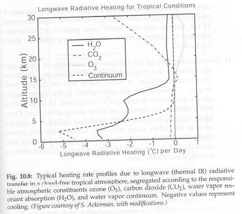
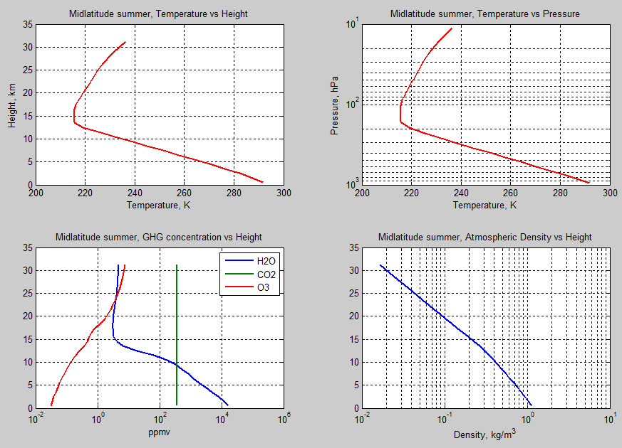
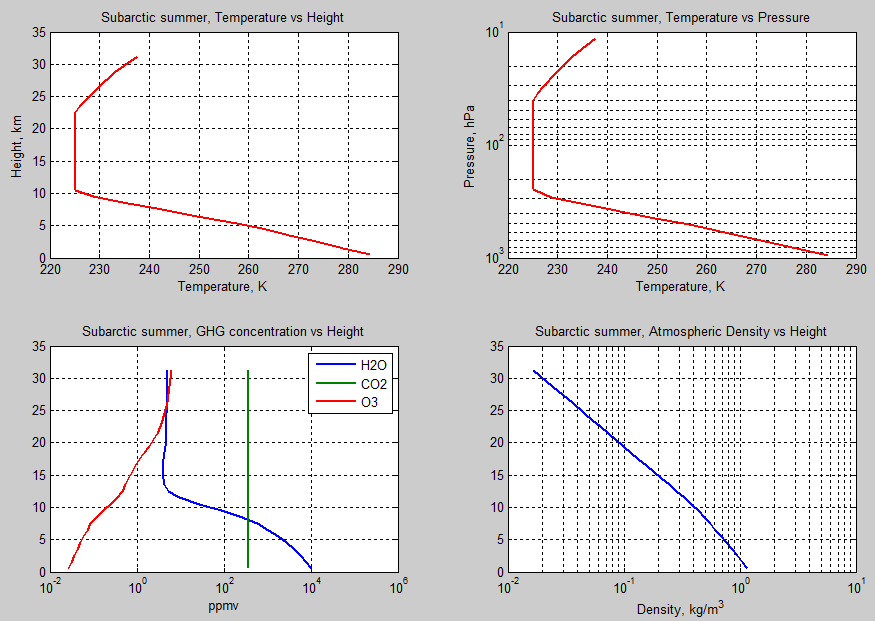
c)  ii) Use one of six standard atmospheres (AFGL) – more info in Part Twelve – Heating Rates

4. Calculate optical thickness for each layer at each wavenumber. dv defines the spacing for the calculation.

For each layer, get each absorption line of each GHG:

– then calculate the actual strength from the line shape equation at each wavenumber of interest across the whole band

– calculate delta tau from that line at that wavenumber and add it to tau(layer,wavenumber)

5. Initialize surface upwards radiation from temperature of surface & emissivity, downward from TOA to be zero.

Calculate transmission through each layer plus emission from each layer to get spectrum at each boundary in both directions.

• Transmissivity = exp(-tau)
• Absorptivity= 1-exp(-tau); Beer Lambert law
• Emissivity = Absorptivity; from Kirchhoff

The above values are for each wavenumber.

6. If more than tstep>2 the change in temperature will be calculated at each layer from change in energy. dT = (change in upward flux through layer + change in downward flux through layer) x timestep / (rho x cp x thickness of layer). It’s just the first law of thermodynamics.

Then convective adjustment checks whether the lapse rate is too great, which is unstable, and if so, adjusts the temperature back to the lapse rate. This critical lapse rate can be different at different heights, currently it is set to one value.

Code

==== v 0.10.4 ====== added to article Jan 30th ===

function [ vt tau fluxu fluxd neth z dz p rho mix zb pb Tb …
Tinit T Ts dE dEs dCE radu radd emitu sheat surfe TOAe rf radupre raddpre …
radupost raddpost TOAf TOAtr alr] =…
HITRAN_0_10_4(dv, std_atm, numz, ratiodp, mol, mixc, newmix, ison, blp, BLH, FTH, STaH, contabs,…
linewon, Tsi, lapsekm, lapseikm, ptropo, minp, ocd, src, tstep, nt, ntc, ploton)
% Radiative transfer through atmosphere, up and down
% Uses the HITRANS database for absorption and emission lines with
% Lorenzian broadening, not yet using Voigt profile; Pierrehumbert 2010 for
% continuum absorption.
% Generally creates a standard atmosphere of pressure, temperature to
% calculate up and down spectral fluxes
% Can work from starting point to recalculate new temperature profile via
% “radiative convective” model using the defined lapse rate
%
%
% v0.1 – Basic calculations to get out of the starting blocks
% v0.2 – Tidy up and allow a “slab” to be at any pressure and temperature
% with line width determined by the pressure & temperature
% v0.3 – Allow multiple layers
% v0.4 – Orphan branch to evaluate wings of lines vs weak lines
% v0.5 – More GHGs, select which ones to pull data in
% v0.6 – Orphan branch not used here, adds CFC-11 & 12 which was difficult
% because the minor GHGs are in a different database
% v0.7 – Dec 31st 2012, significant update to calc emission and absorption
% through atmosphere (rather than just calc transmissivity) as a
% radiative-convective model
% v0.7.1- Added the energy absorbed/emitted by layer/wavenumber from
% rte_0_5_3
% v0.8 – Set boundary layer top pressure so changes to no of layers doesn’t
% alter calcs (BLH can be different from FTH), fix stratosphere temp
% in lieu of solar heating (via iso_strato parameter)
% v0.9 – Introduce continuum absorption of water vapor
% v0.9.1- Adding some interim calcs like effective emission height, % of
% emitted flux from each height that makes up TOA; likewise for DLR;
% v0.9.2- Clean up code comments for publishing, fix the calculation of
% layers just above the boundary layer (as noted by Frank), change
% surface pressure to 1013hPa, fixed convective adjustment to include
% the surface to first atmospheric layer, add different lapse rate
% for each layer
% v0.9.3- Allow stratosphere temp to move, but stay isothermal
% v0.9.4- Orphan version
% v0.9.5- Minor improvements and code efficiency suggested by Pekka
% v0.9.6- Change to input parameters to tidy up code – “mol” is a vector of
% the HITRAN molecule numbers, to match vector “mix” which is the
% matching mixing ratio. This avoids editing code when different
% GHGs are considered.
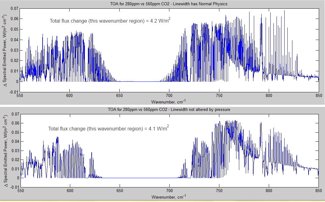
% v0.9.7- Added option to turn off line width formula, primarily to show
% what happens when no narrowing of lines due to pressure (or
% temperature changes)
% v0.10- Better tracking of heat movement when model run to equilibrium
% Removed a few unnecessary variables passed back from function,
% added comments for all variables passed back, note – Ts => Tsi in
% this version
% v0.10.1- Added very basic parameterized solar heating by level, otherwise
% other tradeoffs have to be made (e.g.,lose isothermal statrosphere)
% v0.10.2- Now create new GHG conditions, newmix, at time, ntc. Use (via
% separate function “optical_2” better diffusivity calculation)
% v0.10.3- New layer model, previously the pressure difference for each
% layer was equal, now allow this to change for extending better
% into the stratosphere
% v0.10.4- Further layer model changes – can use one of 6 std atmospheres,
% make GHG concentration now a function of level

% ====== Input conditions (passed to function) ====================
% dv = resolution of wavenumber for calculations in cm^-1
% std_atm = 1-6 to use tropical; mid-latitude summer/winter; subarctic
% summer/winter; US std 1976; *OR* =0 if we define our own from params:
% numz, ratiodp, blp, BLH, FTH, STaH, Tsi, lapseikm, ptropo
% i.e., the above list is NOT used if std_atm>0
% numz = number of boundaries to consider (number of layers = numz-1)
% ratiodp = scaling for the dp across each layer, <=1 (1=each layer the
% same, 0.9 means each layer 10% less pressure than the one before)
% mol = vector of molecule # to be considered from HITRAN numbers: 1=H2O,
% 2=CO2, 3=O3, 4=N2O, 5=CO, 6=CH4, must match mixing ration from
% vector ‘mix’, e.g., mol=[1 2 4 6]; when mix=[0 360e-6 319e-9 1775e-9]
% which means H2O (ignore because set by BLH/FTH), CO2 = 360ppm, N2O
% = 319 ppbv, CH4 = 1775 ppbv
% mixc = mixing ratio for each molecule as described for ‘mol’, but note
% if first value is for H2O it is unused (BLH & FTH are used)
% newmix = new mixing ratio to be introduced (as step function for now) at
% timestep ntc
% ison = number of isotopes for each GHG, must match ‘mol’: 1 = only the
% main is used), e.g., [1 1 1 1] means first isotopologue for the
% 4 GHGs being; if mol=[1 2 3 4] & ison=[1 3 1 1] then CO2 will be
% considered to the 3rd isotopologue but the others only to first
% blp = boundary layer thickness in Pa
% BLH = relative humidity in the boundary layer
% FTH = relative humidity in the free troposphere (currently layers 2,3..)
% STaH = mixing ratio of water vapor in stratosphere
% contabs = true or false for including the water vapor continuum absorption
% linewon = whether to keep linewidth adjustment on or off (for real
% physics = true, for fake physics = false)
% Tsi = initial surface temperature
% lapsekm = lapse rate in troposphere, K/km
% lapseikm = initial lapse rate in troposphere, K/km, to setup initial temp
% profile
% ptropo = defined tropopause pressure
% minp = top of atmosphere to consider for radiative calcs, in pressure (Pa)
% ocd = ocean depth in m – for running dynamic simulations
% src = average solar absorbed radiation (over surface area of earth)
% tstep = timestep in seconds
% nt = number of timesteps
% ntc = number of timesteps where ‘newmix’ of GHGs is introduced, so ntc < nt
% or, if newmix is not wanted, make ntc>nt and newmix will not be
% invoked
% ploton = whether the plot is run or not – lots of other plots are
% generated via separate programs

% ====== Output variables (returned from function) ====================
% vt(numv) = wavenumber vector
% tau(numz-1,numv) = optical thickness by layer and by wavenumber
% fluxu = upward flux at each boundary
% fluxd = downward flux at each boundary
% neth = net radiative heating rate ‘C/day, each layer
% z(numz-1) = height of each layer
% dz(numz-1) = thickness of each layer
% p(numz-1) = pressure of each layer
% rho(numz-1) = density of each layer
% mix(nmol,numz-1) = mixing ratio of each GHG at each layer
% zb(numz) = height at each boundary
% pb(numz) = pressure at each boundary
% Tb(numz) = temperature at each boundary
% Tinit(numz-1) = starting temperature of each layer
% T(numz-1,nt) = temperature of each atmosphere layer at each time step, T(1,:)=Tinit
% Ts(nt) = temperature of ocean
% dE(numz-1,nt) = change in energy each time step in each layer
% dEs(nt) = change in energy each time step in ocean
% dCE(numz-1,nt) = change in convective heat each time step upward to each
% layer (1=from ocean to atmosphere layer 1)
% radu(numz,numv) = upward flux at each boundary, boundary 1 = surface
% radd(numz-1,numv) = downward flux at each boundary
% emitu(numz-1,numv) = emitted radiation from within each layer, layer 1= first
% atmospheric layer
% sheat(numz-1) = absorbed solar in each layer in W/m^2
% surfe(nt) = net flux at surface each timestep (+ve downward)
% TOAe(nt) = net flux at TOA each timestep (+ve downward)
% rf = radiative forcing – from the TOA flux pre and post change in GHG, =0
% if this condition doesn’t take place (GHG change)
% radupre, raddpre, radupost, raddpost – spectrum up and down pre and post
% GHG change
% TOAf(numz,numv) = TOA flux contributed from each boundary
% TOAtr(numv) = surface radiation transmitted to TOA
% alr(numz-1,nt) = actual lapse rate between each layer at each time step, in K/km

disp(‘ ‘);
disp([‘— New Run v0.10.4 — ‘ datestr(now) ‘ —-‘]);
disp(‘ ‘);

% =========== Basic definitions =====================

% Units in SI unless otherwise noted including all pressure values in Pa
% except for SI, frequency in cm^-1
p0=1.013e5; % std pressure for the HITRANS database in Pa
T0=296; % std temperature for HITRANS database in K
Na=6.02e23; % Avogradro’s number
mair=28.96e-3; % molar mass of air
% mh2o=18.02e-3; % molar mass of water vapor
ems=1.0; % emissivity of surface
cp=1005; % cp (specific heat cap at constant pressure) of air
cpw=4180; % cp of air, J/kg.K
rhow=1000; % density of water, kg/m^3
solaratm=true; % solar heating of the atmosphere, currently very parameterized
convadj=true; % if true, convective adjustment to lapse rate = lapse
convloop=10; % no of times to repeat convective loop to get lapse rate correct
iso_strato=false; % if true, fixed and isothermal stratospheric temperature
% if solaratm is true, this should be set to false
lapse=lapsekm/1000; % lapse rate in K/m
lapsei=lapseikm/1000; % initial lapse rate in K/m
rf=0; %radiative forcing if GHG change
print_layers=false; % if true, prints out z, p, T, rho for each layer
windmax=10000/8; windmin=10000/12; % ‘atmospheric window’ region in wavenumber
% for “curiosity value calculation
% set up a few print strings
if contabs
conttext=’Continuum included’;
else
conttext=’No Continuum’;
end
if convadj
convtext=’With convective adjustment’;
else
convtext=’No convective adjustment’;
end
if linewon
linetext=’ Linewidth depends on p,T; ‘;
else
linetext=’ Constant linewidth; ‘;
end
dbh=false; % debug heat stuff added in 0.9.8, if true print a lot out

% =========== Define wavenumber ranges ==============

vmin=10; % min wavenumber to consider (overall)
vmax=2500; % max wavenumber to consider (overall)
% because absorption lines below the lower boundary (and above the upper
% boundary) can still affect the wavenumbers under consideration we need to
% extend the boundaries of which absorption lines to consider
% rvmin=1; % ratio below lower boundary to consider – not useful for a wide range
% rvmax=1; % ratio above upper boundary to consider

vt=vmin:dv:vmax; % vt = wavenumbers we will calculate optical depth for
numv=length(vt); % number of wavenumbers

% =========== Read in GHG data ======================

fprintf(‘%s’, ‘Loading HITRAN data.. ‘);

% names for the HITRAN molecules up to molecule 6, need to be 3 characters
% each because of how Matlab handles strings
Hmols=[‘H2O’; ‘CO2’; ‘O3 ‘; ‘N2O’; ‘CO ‘; ‘CH4’;];

% atmospheric proportions of HITRAN isotopes up to molecule 6, data from
% Rothman et al (2005) table 6, vector ‘ison’ extracts the values needed
Hisoprop=[0.9973 0.0020 0.0004; 0.9842 0.0111 0.0039; 0.9929 0.0040 0.0020; …
0.9903 0.0036 0.0036; 0.9865 0.0111 0.0020; 0.9883 0.0111 0.0006];

% select data on GHGs from vector “mol”, isotopes to consider, define isotope ratios

% how many molecules are being considered
nmol=length(mol);
% select the molecule names being used from the list in ‘mol’
mols=Hmols(mol,:);
% select isotopologues for each molecule, each molecule, m, will only be
% considered to the depth of ison(m) defined in the function parameters
isoprop=Hisoprop(mol,1:max(ison));

% Now read in the line data via ‘Hitran_read’ function

% v=line position, S=line strength, iso=isotopologue, gama = air-broadened
% half-width, nair=temperature-dependence exponent for gama

% We don’t know the final size of the vectors and some GHGs have very large
% lists, while others are very small so space considerations mean creating
% a [1 x total lines] array rather than [nmol x max of largest]
for i=1:nmol
if i==1 % first value established the vector

[ v S iso gama nair ] = Hitran_read_0_2(mol(i), vmin, vmax, ison(i));
% now set an identifier
molx=ones(1,length(v))*mol(i); % identifies all these values as this molecule

else % now subsequent values get appended
[ v1 S1 iso1 gama1 nair1 ] = Hitran_read_0_2(mol(i), vmin, vmax, ison(i));

molx1=ones(1,length(v1))*mol(i); % identifies all these values as this molecule
v=[v v1]; iso=[iso iso1]; gama=[gama gama1]; S=[S S1]; nair=[nair nair1];
molx=[molx molx1];
end
end

fprintf(‘%s’, ‘finished.. ‘);
% =========== Finished reading GHG data ======================

% =========== Define standard atmosphere against height =============

ps=1.013e5; % define surface pressure

if std_atm>0 % if we want to use one of the 6 AFGL std atmospheres
load(‘AFGL’) % this has height, pressure, temperature and concentrations
% of water vapor, O3, NO2, CH4 – not CO2, set from mixc
numz=find(AFGLp(std_atm,:)<minp,1); % number of boundaries
zb=zeros(1,numz); pb=zeros(1,numz); Tb=zeros(1,numz); rhob=zeros(1,numz);
zb=AFGLz(1:numz); % height of boundaries in meters
pb=AFGLp(std_atm,1:numz); % pressure of boundaries in Pa
Tb=AFGLt(std_atm,1:numz); % temperature of boundaries
Tsi=AFGLt(std_atm,1); % set ocean starting temperature

% calculate pressure, height, temperature, density in midpoint of layer
% [could have used the specified points as the middle of layers but need
% some consistency with the existing calculation of atmospheres]
dz=zeros(1,numz-1);z=zeros(1,numz-1);Tinit=zeros(1,numz-1);
p=zeros(1,numz-1);rho=zeros(1,numz-1);
mix=zeros(nmol,numz-1); % matrix of mixing ratios for molecule, height

p=(pb(2:numz)+pb(1:numz-1))/2; % pressure in midpoint of layer
Tinit=(Tb(2:numz)+Tb(1:numz-1))/2; % initial temperature in midpoint of layer
z=(zb(2:numz)+zb(1:numz-1))/2; % height in midpoint of layer
rho=p./(Tinit*287); % density in midpoint of layer in kg/m^3 from ideal gas law
dz=zb(2:numz)-zb(1:numz-1);

% Create matrix ‘mix'(each molecule,each height)
loch2o=find(mol==1, 1); % location in mol vector of H2O
if ~(isempty(loch2o)) % if water vapor used
% water vapor in mid-point of boundary
mix(loch2o,:)=(AFGLh2o(std_atm,1:numz-1)+AFGLh2o(std_atm,2:numz))/2;
end
locco2=find(mol==2, 1); % location in mol vector of CO2
if ~(isempty(locco2)) % if CO2 is used
mix(locco2,:)=mixc(locco2); % set the concentration of CO2 at all heights the same
end
loco3=find(mol==3, 1); % location in mol vector of O3
if ~(isempty(loco3)) % if O3 is used
% set the concentration of O3 to that atmosphere
mix(loco3,:)=(AFGLo3(std_atm,1:numz-1)+AFGLo3(std_atm,2:numz))/2;
end
locn2o=find(mol==4, 1); % location in mol vector of N2O
if ~(isempty(locn2o)) % if N2O is used
% set the concentration of N2O to that atmosphere
mix(locn2o,:)=(AFGLn2o(std_atm,1:numz-1)+AFGLn2o(std_atm,2:numz))/2;
end
locch4=find(mol==6, 1); % location in mol vector of CH4
if ~(isempty(locch4)) % if CH4 is used
% set the concentration of CH44 to that atmosphere
mix(locch4,:)=(AFGLch4(std_atm,1:numz-1)+AFGLch4(std_atm,2:numz))/2;
end
% are needed ptropo & iztropo needed – not defined with std atmospheres?

else % we want to create our own atmosphere based on the surface temperature,
% Tsi, the lapse rate, lapsekm, boundary layer pressure, blp

% —- First create a “high resolution” atmosphere
% zr = height, pr = pressure, Tr = temperature, rhor = density

maxzr=50e3; % height of high resolution atmosphere
numzr=5001; % number of points used to define high res. atmosphere
zr=linspace(0,maxzr,numzr); % height vector from sea level to maxzr

% use ‘define_atmos’ function to determine pr, Tr, rhor & ztropo (height of
% tropopause)
[pr Tr rhor ztropo] = define_atmos_0_5(zr,Tsi,ps,ptropo,lapsei);
% for consideration – if the radiative-convective model changes temperature
% significantly, should the pressure be re-adjusted?

% —- Second, create “coarser resolution” atmosphere – this reduces
% computation requirements for absorption & emission of radiation
% – this atmosphere has numz boundaries and numz-1 layers

% z, p, Tinit, rho; subset of values used for RTE calcs

% We divide the atmosphere into either approximately equal pressure changes
% or reduce dp for each successive layer by factor ratiodp
% Note: first layer is the boundary layer at pressure = blp
% with different humidity (BLH)

zi=zeros(1,numz); % zi = lookup vector to “select” heights, pressures etc
zi(1)=1; % make first value the surface value
zi(2)=find(pr<=blp, 1); % gets the location of boundary layer top edge
dptot=blp-minp;

if ratiodp==1 % if equal pressure change for each layer
dp=dptot/(numz-2); % finds the pressure change for each height change

for i=3:numz % locate each value
zi(i)=find(pr<=(pr(zi(2))-(i-2)*dp), 1); % gets the location in the vector where
% pressure is that value
end
elseif ratiodp<1 && ratiodp>0 % if progressively reduced pressure change
dp=(dptot*(1-ratiodp))/(1-ratiodp^(numz-2)); % calculate value of dp to
% meet the total pressure change with this geometric series & ratiodp
ptemp=zeros(1,numz);ptemp(1)=ps;ptemp(2)=blp;
for i=3:numz
ptemp(i)=ptemp(i-1)-dp*ratiodp^(i-3);
zi(i)=find(pr<=ptemp(i),1);
end

else % bad parameter
disp(‘Error, ratiodp must be >0 && <=1′);
return
end

% now create the vectors of coarser resolution atmosphere
% zb is height of boundaries, zb(1) = surface; zb(numz) = TOA
% T, p, rho are all the midpoint (pressure) between the boundaries

zb=zr(zi); % height at boundaries
pb=pr(zi); % pressure at boundaries
Tb=Tr(zi); % starting temperature at boundaries
rhob=rhor(zi); % density at boundaries

% now calculate density, pressure, temperature and water vapor saturation
% mixing ratio at midpoint of each layer – midpoint by pressure
dz=zeros(1,numz-1);z=zeros(1,numz-1);Tinit=zeros(1,numz-1);
p=zeros(1,numz-1);rho=zeros(1,numz-1);
im=zeros(1,numz-1); % index for getting midpoints at midpoint pressure

% calculate pressure in midpoint of layer
for i=1:numz-1
p(i)=(pb(i+1)+pb(i))/2; % pressure in midpoint of layer
dz(i)=zb(i+1)-zb(i); % thickness of each layer
end

% lookup midpoint values for z, T, rho at the midpoint pressure
for i=1:numz-1
im(i)=find(pr<=p(i), 1); % gets the location in the vector of midpoint pressure
end

z=zr(im); % calculate height of midpoint pressure
Tinit=Tr(im); % temperature of midpoint pressure
rho=rhor(im); % density of midpoint pressure
iztropo=find(pb<ptropo,1)-1; % location in the p vector of the first layer above the tropopause

% now copy the vector mixc to each height
mix=repmat(mixc’,1,numz);
% now calc mixing ratio in molecules for water vapor at prescribed RH
for i=1:numz-1
% = RH * es / p
% currently satvaph2o() gives es=610.94.*exp(17.625.*Tc./(Tc+243.04)); where Tc in ‘C
if i==1
mix(1,i)=BLH*satvaph2o(Tinit(i))/p(i);
elseif i<iztropo
mix(1,i)=FTH*satvaph2o(Tinit(i))/p(i);
else
mix(1,i)=STaH;
end
end
end

% calculate Heat capacity for each layer, Cp = rho x dz x cp in J/K
Cp=zeros(1,numz-1);
Cp=rho.*dz.*cp; % of each atmospheric layer
Cps=rhow*ocd*cpw; % of ocean

lapsez=ones(1,numz-1)*lapse; % lapse rate for convective adjustment can be
% different for each layer, current all set to ‘lapse’
radupre=zeros(numz,numv);radupost=zeros(numz,numv); % create matrix for some spectral
raddpre=zeros(numz,numv);raddpost=zeros(numz,numv); % values, that only get assigned
% if a jump in GHGs

% ———— Solar Heating of the Atmosphere

sheat=zeros(1,numz-1); % W/m^2 solar heating of each layer of the atmosphere
sheath2o=zeros(1,numz-1); % W/m^2 solar heating by water vapor of each layer of the atmosphere

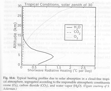
if solaratm % if we are using solar heating of the atmosphere
% ozone and water vapor, first pass, using solar heating rates from
% Petty (2006), p.313
% first ozone, use 0’C/day at 10km, straight line through 2’C/day at
% 30km and convert to W/m^2
sheat=(z>=10000).*((z./1000-10)/7).*Cp/86400;
%sheat=(z>=10000).*((z./1000-10)/10).*Cp/86400;
% now water vapor – this will be the most badly modeled due to the
% variability of water vapor – convert to W/m^2
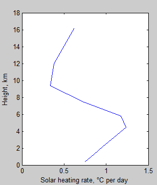
sheath2o=(((z<5000).*(z./1000*.6/5+.7))+(z>=5000 & z<9000).*((9000-z)./1000*1.1/4+.3)…
+(z>=9000 & z<15000).*((15000-z)./1000*.3/5)).*Cp/86400;
sheat=sheat+sheath2o;
end

if print_layers % display values at each pressure
disp(‘ ‘);
if std_atm==0
disp([‘dp= ‘ num2str(dp)]);
disp([‘Pressure of tropopause layer = ‘ num2str(z(iztropo)) ‘, at ‘ num2str(iztropo)]);
end
for i=1:numz-1
disp([‘p= ‘ num2str(p(i)/100,’%4.0f’) ‘, z= ‘ num2str(z(i),’%4.0f’)…
‘, T= ‘ num2str(Tinit(i)) ‘, rho= ‘ num2str(rho(i),’%4.2f’)]);
end
% for i=1:numz
% disp([‘pb= ‘ num2str(pb(i)/100,’%4.0f’) ‘, z= ‘ num2str(zb(i),’%4.0f’)]);
% end
end

% =========== Finished defining standard atmosphere against height ======
% =========== Absorption and Emission – each layer of the atmosphere, i =====
% note: work in cm for volumes and distances (absorption coefficients are in cm)

% call optical thickness for each layer of the atmosphere
% this function can be repeated if GHGs change (or temperature changes)
% have to pass the atmospheric layers (p, T, rho, mix, numz-1), the
% HITRAN data (v, S, iso, gama, nair) and the GHG concentrations (mix,
% ison)

tau=optical_3(vt, v, S, iso, gama, nair, molx, numz, numv, p, p0, Tinit, …
T0, Na, rho, mair, dz, mol, nmol, mix, isoprop, contabs, linewon);
% now calculate the transmissivity and absorptivity for each layer and
% wavenumber
% i = layer, k = wavenumber
tran=zeros(numz-1,numv); abso=zeros(numz-1,numv); % set array
for i=1:numz-1 % each layer
for k=1:numv % each wavenumber interval
tran(i,k)=exp(-tau(i,k)); % transmissivity = 0 – 1
abso(i,k)=(1-tran(i,k)); % absorptivity = emissivity = 1-transmissivity
end
end

% =========== Calculate absorption, emission & temperature changes =========

Ts=zeros(1,nt); % define array to store ocean temperature
T=zeros(numz-1,nt); % define array to store T for each atmospheric level and time step
dEs=zeros(1,nt); % energy change for ocean for each time step
dE=zeros(numz-1,nt); % energy change for each atmospheric level
dCE=zeros(numz-1,nt); % convective energy tracking

sr=ones(1,nt)*src; % solar flux at TOA vs time (later can vary with time)
sr0=sr-sum(sheat); % define solar flux absorbed at surface (=solar at
% TOA – atmospheric absorbed)

T(:,1)=Tinit; % load temperature profile for start of scenario
Ts(1)=Tsi; % ocean temperature for first time step (this could have been the bottom
% layer of the atmospheric model, but feature added after code developed

TOAe=zeros(1,nt); % TOA instantaneous flux balance vs time
surfe=zeros(1,nt); % Surface instantaneous flux balance vs time

% =========== Main loops to calculate TOA spectrum & flux =====

% first, we timestep
% second, we work through each layer
% third, through each wavenumber
% fourth, through each absorbing molecule
% currently calculating surface radiation absorption up to TOA AND
% downward radiation from TOA (at TOA = 0)

% h = timestep, i = layer, j = wavenumber
for h=2:nt % main iterations to achieve equilibrium
if dbh
disp([‘Timestep ‘ num2str(h)]);
%fprintf(‘%d %s’, h, ‘ ‘); % display current timestep being calculated
end

if h==ntc % change to GHG concentrations, currently keep water vapor
% concentration the same and use same temperature as
% starting conditions

tau=optical_3(vt, v, S, iso, gama, nair, molx, numz, numv, p, p0, Tinit,…
T0, Na, rho, mair, dz, mol, nmol, newmix, isoprop, contabs, linewon);

% now calculate the transmissivity and absorptivity for each layer and
% wavenumber
% i = layer, k = wavenumber
tran=zeros(numz-1,numv); abso=zeros(numz-1,numv); % set array
for i=1:numz-1 % each layer
for k=1:numv % each wavenumber interval
tran(i,k)=exp(-tau(i,k)); % transmissivity = 0 – 1
abso(i,k)=(1-tran(i,k)); % absorptivity = emissivity = 1-transmissivity
end
end
end

radu=zeros(numz,numv); % initialize upward intensity at each *boundary* and wavenumber
radu1=zeros(numz,numv); % initialize curiosity version of radu (no emission)
emitu=zeros(numz-1,numv); % initialize emission upward for each *layer* and wavenumber

radd=zeros(numz,numv); % initialize downward intensity at each *boundary* and wavenumber
emitd=zeros(numz-1,numv); % initialize emission downward for each *layer* and wavenumber
radu(1,:)=ems.*planckmv(vt,Ts(h-1)); % upward *surface* radiation vs wavenumber
radu1(1,:)=radu(1,:); % evaluating radiation transfer with no emission – for interest
radd(end,:)=zeros(1,numv); % downward radiation at TOA vs wavenumber (=zero)
% units of radu, radd, emitu, emitd are W/m^2.cm^-1, i.e., spectral emissive power

% Upwards spectral emissive power
for i=1:numz-1 % each layer
for j=1:numv % each wavenumber interval

% calc intensity (each wavenumber) at next boundary
% = incoming * transmissivity + emission
% emission upward = Planck formula x emissivity (=absorptivity)
emitu(i,j)=abso(i,j)*3.7418e-8.*vt(j)^3/(exp(vt(j)*1.4388/T(i,h-1))-1);
% calculate spectral emissive power at next upward boundary
radu(i+1,j)=radu(i,j)*tran(i,j)+emitu(i,j);
radu1(i+1,j)=radu1(i,j)*tran(i,j); % transmitted only, for curiosity

% Change in radiated energy = dI(v) * dv (per second)
% accumulate through each wavenumber
% if the upwards radiation entering the layer is more than
% the upwards radiation leaving the layer, then a heating
dE(i,h)=dE(i,h)+(radu(i,j)-radu(i+1,j))*dv*tstep;
% pre 0.10; Eabs(i)=Eabs(i)+(radu(i,j)-radu(i+1,j))*dv;
end % each wavenumber interval
end % each layer

% Downwards spectral emissive power
for i=numz-1:-1:1 % each layer from the top down
for j=1:numv % each wavenumber interval
% calculate emission downward (same as upward but in case we
% play around later)
emitd(i,j)=abso(i,j)*3.7418e-8.*vt(j)^3/(exp(vt(j)*1.4388/T(i,h-1))-1);
% calculate spectral emissive power at next upward boundary
radd(i,j)=radd(i+1,j)*tran(i,j)+emitd(i,j);
dE(i,h)=dE(i,h)+(radd(i+1,j)-radd(i,j))*dv*tstep;
end % each wavenumber interval
dE(i,h)=dE(i,h)+sheat(i)*tstep; % add in solar absorbed for this layer

dT=dE(i,h)/Cp(i); % change in temperature = dQ/heat capacity
if dbh
disp([‘Layer ‘ num2str(i) ‘, dE = ‘ num2str(dE(i,h)) ‘, dT= ‘ num2str(dT)]);
end

if iso_strato && i>iztropo % if we want to keep stratosphere at fixed temperature
% but allow whole stratosphere temp to move in this version,
% defined by the value of temperature in the tropopause layer
T(i,h)=T(iztropo,h-1); % layers above fixed to last iteration of tropopause layer
% calculating from top down so can’t use current time period value

% **** need to account for movement of heat in this part of the
% atmosphere under this scenario – not yet done
else
T(i,h)=T(i,h-1)+dT; % calculate new temperature

if T(i,h)>500 % picks up finite element problem
disp([‘Terminated at h= ‘ num2str(h) ‘, z(i)= ‘ num2str(z(i)) ‘, i = ‘ num2str(i)]);
disp([‘time = ‘ num2str(h*tstep/3600) ‘ hrs; = ‘ num2str(h*tstep/3600/24) ‘ days’]);
disp(datestr(now));
return
end
end
% might need a step to see how close to an equilibrium we are
% getting – not yet implemented because this part of routine is so fast
end % each layer

% now ocean heat changes (via radiation) = time x (Solar + Rdown -Rup)
dEs(h)=(sr0(h)+(sum(radd(1,:))-sum(radu(1,:)))*dv)*tstep;
% Temperature change = Energy change / Cp
Ts(h)=Ts(h-1)+ dEs(h)/Cps;
if dbh
disp([‘Ocean dE = ‘ num2str(dEs(h)) ‘, new Ts= ‘ num2str(Ts(h))]);
end

% now apply convective adjustment
if convadj==true % if convective adjustment chosen..

for j=1:convloop % we need to iterate to a solution
tc=zeros(1,numz-1); % temporary value of convective energy

% Have already worked out the new temperatures for timestep,h,
% based on radiated energy from previous time step, so use this
% timestep and adjust for convection
% Problem is 3 simultaneous equations with 3 unknowns because both
% the temperature above and below change and the lapse rate must be
% valid for the new temperatures

% First from surface to layer 1, slightly different code
if (Ts(h)-T(1,h))/z(1)>lapsez(1) % if lapse rate is too high

tc(1)=(Ts(h)-T(1,h)-z(1)*lapsez(1))/(1/Cps+1/Cp(1));
if tc(1)<0 % should always be positive ***
disp([‘Error in convective adj. layer 1, h= ‘ num2str(h)…
‘, i= ‘ num2str(i) ‘, dCE= ‘ num2str(tc(1))]);
end

if dbh
disp([‘Lapse to layer 1= ‘ num2str((Ts(h)-T(1,h))/z(1)*1000) ‘K/km, newT= ‘…
num2str(newT) ‘, old atm T= ‘ num2str(T(1,h)) ‘, T(ocean)= ‘ num2str(Ts(h))]);
end

dEs(h)=dEs(h)-tc(1); % reduce heat tracking stored in ocean
dE(1,h)=dE(1,h)+tc(1); % increase heat tracking stored in atmos layer 1
T(1,h)=T(1,h)+tc(1)/Cp(1); % calc revised atmospheric temperature
Ts(h)=Ts(h)-tc(1)/Cps; % calc revised ocean temperature

end
% Now for all the atmospheric layers
for i=2:numz-1
if (T(i-1,h)-T(i,h))/(z(i)-z(i-1))>lapsez(i) % too cold, convection will readjust
% calculate the convective heat transfer that satisfies the
% simulataneous equation
tc(i)=(T(i-1,h)-T(i,h)-(z(i)-z(i-1))*lapsez(i))/(1/Cp(i)+1/Cp(i-1));

if tc(i)<0 % should always be positive ***
disp([‘Error in atm convective adj, h= ‘ num2str(h)…
‘, i= ‘ num2str(i) ‘, dCE= ‘ num2str(tc(i))]);
end
if dbh
disp([‘Lapse from layer ‘ num2str(i) ‘ to ‘ num2str(i-1)…
‘ = ‘ num2str((T(i-1,h)-T(i,h))/(z(i)-z(i-1))*1000) ‘ K/km, newT= ‘ …
num2str(newT) ‘, old atm T= ‘ num2str(T(i,h))]);
end

dE(i-1,h)=dE(i-1,h)-tc(i); % reduce heat tracking stored in layer below
dE(i,h)=dE(i,h)+tc(i); % increase heat tracking stored in this layer
T(i,h)=T(i,h)+tc(i)/Cp(i); % set revised atmospheric temperature
% also adjust atmospheric layer below (has lost heat)
T(i-1,h)=T(i-1,h)-tc(i)/Cp(i-1);

end
end
% now accumulate the convective adjustments
dCE(:,h)=dCE(:,h)+tc’;
end
end

% instantaneous imbalance at TOA (+ve downward) in W/m^2 = (solar rate – olr rate)
TOAe(h)=sr(h)-sum(radu(numz,:))*dv;
% instantaneous imbalance at surface in W/m^2 +ve downward = solar + DLR – Surface
% emitted – convected (per second)
surfe(h)=sr0(h)+sum((radd(1,:))-radu(1,:))*dv-dCE(1,h)/tstep;

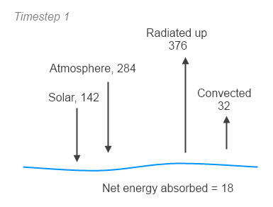
% 1st law of thermodynamics check; heat gained = Es +sum(E)
dqgain=dEs(h)+sum(dE(:,h)); % net energy absorbed in the time step
if abs(TOAe(h)*tstep-dqgain)>1 % if more than 1W discrepancy
disp([‘Time step ‘ num2str(h) ‘, Net Energy missing = ‘ num2str(TOAe(h)*tstep-dqgain)]);
end

% if 1st or middle timestep, or just before & after change in GHGs..
if h==2
% print out initial results of flux
disp([‘ Time= ‘ num2str(h*tstep/86400,’%4.2f’) ‘ days, Flux up at TOA = ‘…
num2str(sum(radu(end,:))*dv,’%4.1f’) ‘ W/m^2, Flux down at surface = ‘ …
num2str(sum(radd(1,:))*dv,’%4.1f’) ‘ W/m^2’]);
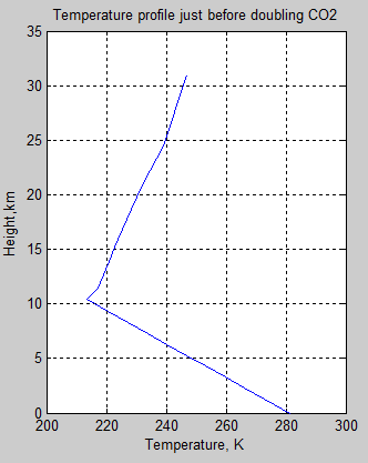
elseif h==ntc-1
% display values
disp([‘ Just before GHG change: time= ‘ num2str(h*tstep/86400,’%4.2f’)…
‘ days, Flux up at TOA = ‘ num2str(sum(radu(end,:))*dv,’%4.1f’)…
‘ W/m^2, Flux down at surface = ‘ num2str(sum(radd(1,:))*dv,’%4.1f’) ‘ W/m^2’]);
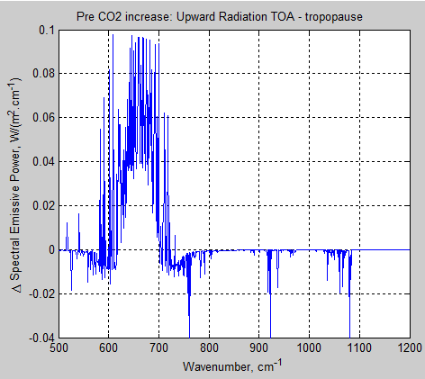
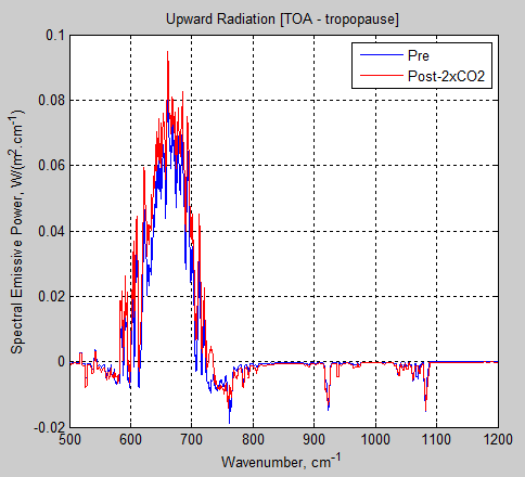
% capture upwards and downwards spectrum
raddpre=radd;radupre=radu;
elseif h==ntc
disp([‘ Just after GHG change: time= ‘ num2str(h*tstep/86400,’%4.2f’)…
‘ days, Flux up at TOA = ‘ num2str(sum(radu(end,:))*dv,’%4.1f’)…
‘ W/m^2, Flux down at surface = ‘ num2str(sum(radd(1,:))*dv,’%4.1f’) ‘ W/m^2’]);
rf=TOAe(ntc-1)-TOAe(h); % radiative forcing from the change
disp([‘Pseudo radiative forcing= ‘ num2str(rf,’%4.1f’) ‘ W/m^2’]);
disp(‘ ‘);
% capture upwards and downwards spectrum
raddpost=radd;radupost=radu;
end
end % —- timestep iterations

% =========== Finish loops to calculate TOA spectrum, flux =====

% Calculate TOA and DLR flux
fluxu=sum(radu’)*dv; % calculate the final up flux at each boundary
fluxd=sum(radd’)*dv; % calculate the final down flux at each boundary

% Calculate heating rates
neth=86400*(diff(fluxd)-diff(fluxu))./Cp; % +ve number = heating, ‘C/day

% =========== Calculate some curiosity values ===============

% flux transmitted from surface and in “atmospheric window”
% calculate the surface radiation transmitted to TOA (integral with dv)
TOAtr=dv*radu(1,:)*exp(-sum(tau))’;
iw=find(vt>=windmin & vt<=windmax); % find the window region in the vector

% flux proportions transmitted from each layer & from the surface, by
% wavenumber
stau=zeros(numz-1,numv); % optical thickness by wavenumber summed from top down
TOAf=zeros(numz,numv); % TOA flux proportion, has to include surface so is number of layers + 1
TOAf(numz,:)=dv*emitu(numz-1,:); % get the top layer, no attenuation
stau(numz-1,:)=tau(numz-1,:); % set the first tau value for the top layer

for i=numz-2:-1:1
% flux from layer i+1 transmitted to TOA is emitu(i)*stau(i+1)
% needed to shift everything up 1 layer so that the surface can be
% included
TOAf(i+1,:)=dv*emitu(i,:).*exp(-stau(i+1,:));
% sum tau going downwards
stau(i,:)=stau(i+1,:)+tau(i,:); %
end
TOAf(1,:)=dv*radu(1,:).*exp(-stau(1,:)); % radu(1,:)= surface intensity (below the bottom layer of atmosphere)

% Calculate the lapse rates for each layer at each timestep
alr=zeros(numz-1,nt);
alr(1,:)=1000*(Ts-T(1,:))./z(1); % ocean to layer 1
for i=2:numz-1
alr(i,:)=1000*(T(i-1,:)-T(i,:))./(z(i)-z(i-1)); % value in K/km
end

% Print out inputs to simulation
disp(‘ ‘); % to produce a newline
if std_atm==0 % if user designed profile

disp([‘Tsi= ‘ num2str(Tsi) ‘, Lapse rate= ‘ num2str(lapsekm) ‘, ‘ conttext ‘, BLH= ‘ num2str(BLH*100)…
‘%, FTH= ‘ num2str(FTH*100) ‘%, blp = ‘ num2str(blp/100) ‘hPa, TOA = ‘ num2str(minp/100) ‘hPa’]);
disp([num2str(numz-1) ‘ layers, dv= ‘ num2str(dv) ‘cm-1, ‘ linetext num2str(nt) …
‘ timesteps of ‘ num2str(tstep/3600/24,’%4.2f’) ‘ days’]);
disp([‘Solar absorbed= ‘ num2str(src) ‘ W/m^2, Absorbed in atmosphere= ‘ …
num2str(sum(sheat),’%4.2f’) ‘ W/m^2’]);
disp(convtext);

else % using a std atmosphere
disp([‘Using AFGL ‘ AFGLname(std_atm,:)]);
disp([‘Surface temperature= ‘ num2str(Tsi) ‘ K, TOA = ‘ num2str(minp/100) ‘hPa’]);
disp([num2str(numz-1) ‘ layers, dv= ‘ num2str(dv) ‘cm-1, ‘ linetext num2str(nt) …
‘ timesteps of ‘ num2str(tstep/3600/24,’%4.2f’) ‘ days’]);
disp([‘Solar absorbed= ‘ num2str(src) ‘ W/m^2, Absorbed in atmosphere= ‘ …
num2str(sum(sheat),’%4.2f’) ‘ W/m^2’]);
disp([convtext ‘, ‘ conttext]);
end

% Print out GHG concentrations
for i=1:nmol
if mol(i)>1 % i.e. is not water vapor, which is printed via BLH, FTH
fprintf([mols(i,:) ‘= ‘ num2str(mix(i)*1e6) ‘ ppm, ‘],’%s’);
end
end
disp(‘ ‘);

% Print out various flux values
disp(‘ ‘);
disp([‘ Final Time= ‘ num2str(h*tstep/86400,’%4.2f’) ‘ days’]);
disp([‘Flux up at TOA = ‘ num2str(fluxu(numz),’%4.1f’) ‘ W/m^2, Flux down at surface = ‘ …
num2str(fluxd(1),’%4.1f’) ‘ W/m^2’]);
disp([‘TOA transmitted surface flux= ‘ num2str(TOAtr,’%4.1f’) ‘ W/m^2, Surface emission= ‘ …
num2str(sum(radu(1,:)),’%4.1f’) ‘ W/m^2, Window transmission= ‘ …
num2str(sum(radu1(numz,iw))/sum(radu(1,iw))*100,’%4.1f’) ‘ %’]);
disp([‘Starting flux imbalance TOA= ‘ num2str(TOAe(2),’%4.2f’) ‘ W/m^2, Final imbalance TOA= ‘ …
num2str(TOAe(end),’%4.2f’) ‘ W/m^2’]);

% Print out temperature values & lapse rate
disp(‘ ‘);
disp(‘Temperature change, start to finish ‘);
for i=numz-1:-1:1
disp([‘Layer ‘ num2str(i) ‘ = ‘ num2str(T(i,nt)-T(i,1),’%4.2f’)]);
end
disp([‘Temp change ocean = ‘ num2str(Ts(nt)-Ts(1),’%4.2f’)]);
disp(‘Final lapse rate ‘);
for i=numz-1:-1:2
disp([‘Lapse rate ‘ num2str(i-1) ‘-‘ num2str(i) ‘ = ‘ …
num2str(alr(i,end),’%4.2f’) ‘ K/km’]);
end
disp([‘Lapse rate ocean – 1 = ‘ num2str(alr(1,end),’%4.2f’) ‘K/km’]);

% =========== Plots, if needed ==================
if ploton

% ====== Graphs vs time – Temperature different layers, TOA & surface
% forcing energy change each layer, convective energy
figure(1)
tv=2:nt; % time vector, a lot of values are first calculated on timestep 2

iz=[1 4 8 12 16 20]; % atmospheric layers to consider (to reduce graph clutter)
nump=length(iz); % number of items plotted

% Create relevant graph legends for the selected layers
textleg(1)={‘Ocean’};
for i=1:nump
textleg(i+1)={[num2str(iz(i))]};
end
nump=length(iz); % number of items plotted
textleg1(1)={[‘Ocean->’ num2str(iz(1))]};
for i=2:nump
textleg1(i)={[num2str(iz(i)-1) ‘-‘ num2str(iz(i))]};
end

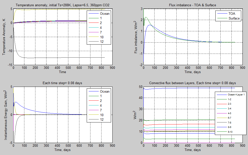
% 1. Temperature anomaly vs time
subplot(2,2,1),plot((1:nt)*tstep/86400, Ts-Ts(1), …
(1:nt)*tstep/86400, T(iz,:)-(repmat(T(iz,1),1,nt)))
ylabel(‘Temperature Anomaly, K’)
xlabel(‘Time’)
title([‘Temperature anomaly, initial Ts=’ num2str(Tsi),’K, Lapse=’ num2str(lapsekm)])
grid on
%legend(‘Ocean’,’1′,’2′,’3′,’4′,’5′,’6′,’7′,’8′,’9′, ’10’)
legend(textleg);

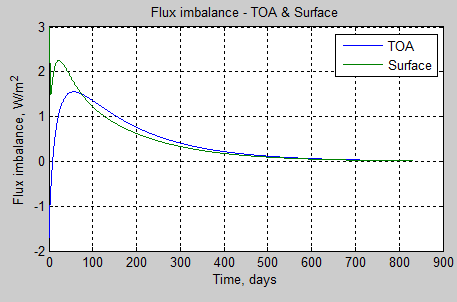
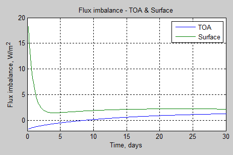
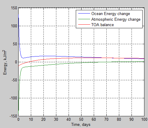
% 2. TOA & surface imbalance vs time
subplot(2,2,2),plot(tv*tstep/86400,TOAe(tv),tv*tstep/86400,surfe(tv))
xlabel(‘Time, days’)
ylabel(‘Flux imbalance, W/m^2’)
grid on
legend(‘TOA’,’Surface’)

% 3. Energy change each layer vs time (converted to instantaneous)
subplot(2,2,3),plot(tv*tstep/86400,dEs(tv)/tstep,tv*tstep/86400,dE(iz,tv)/tstep)
xlabel(‘Time, days’)
ylabel(‘Instantaneous Energy Gain, W/m^2’)
title([‘Each time step= ‘ num2str(tstep/86400,’%3.2f’) ‘ days’])
grid on
legend(textleg);

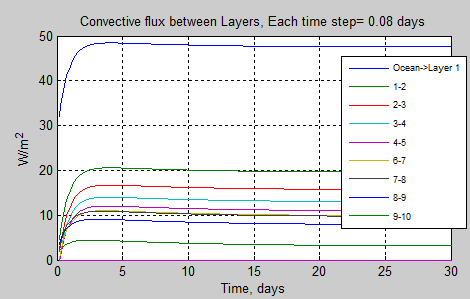
% 4. Convective flux between layers vs time
subplot(2,2,4),plot(tv*tstep/86400,dCE(iz,tv)/tstep)
xlabel(‘Time, days’)
ylabel(‘W/m^2’)
grid on
title([‘Convective flux between Layers, Each time step= ‘ num2str(tstep/86400,’%3.2f’) ‘ days’])
legend(textleg1);

% ====== Cumulative transmitted flux to TOA & Emitted flux each layer
figure(2)
% Cumulative transmitted flux to TOA
zz=[0 z]; % add the surface to the height vector to make it possible to plot
zTOA=sum(TOAf’).*dv; % get the integrated value across wavelengths, each boundary
accTOA=zeros(1,numz); % accumulated values
accTOA(1)=zTOA(1);
for i=2:numz
accTOA(i)=accTOA(i-1)+zTOA(i); % calculated accumulated values (as per Part 3 blog comment)
end
subplot(1,2,1),plot(accTOA,zz/1000,’r*’)
xlabel(‘Cumulative flux reaching TOA, W/m^2’)
ylabel(‘Height of layer, km’)
title(‘Cumulative transmitted flux from each layer to TOA’)
grid on
% Emitted flux from each atmospheric layer & surface
% ’emitu’ is from each atmos. layer, we need to add surface
emitted=[sum(radu(1,:))*dv sum(emitu’)*dv];
subplot(1,2,2),plot(emitted,zz/1000,’b*’)
xlabel(‘Emitted flux, W/m^2’)
ylabel(‘Height of layer, km’)
title(‘Emitted flux from each layer’)
grid on

% ====== Plot lapse rate as a check, and temperature profile vs height
figure(3)
% Actual lapse rate – for checking
% Not so useful when past 10 layers, so just the first 9
subplot(1,2,1),plot((1:nt)*tstep/86400,alr(1:10,:))
xlabel(‘Time, days’)
ylabel(‘Lapse rate, K/km’)
title(‘Lapse rate change with time for bottom set of layers’)
grid on
legend(‘Ocean->Layer 1’, ‘1-2′,’2-3′,’3-4′,’4-5′,’5-6’, ‘6-7′,’7-8′,’8-9′,’9-10’)

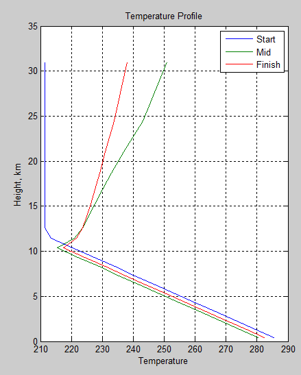
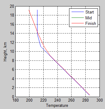
% Vertical temperature profile at 3 times
subplot(1,2,2),plot(T(:,1),z/1000,T(:,ceil(nt/2)),z/1000,T(:,end),z/1000)
legend(‘Start’,’Mid’,’Finish’)
ylabel(‘Height, km’)
xlabel(‘Temperature’)
title(‘Temperature Profile’)
grid on

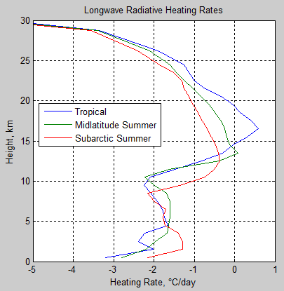
% ======== Plot flux and cooling to space curve

figure(4)
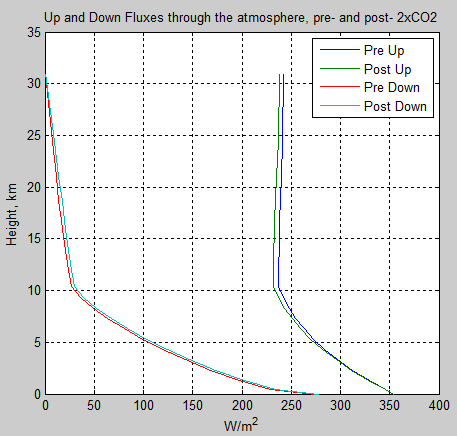
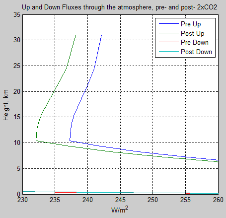
subplot(1,2,1),plot(fluxu,zz/1000,fluxd,zz/1000,’Linewidth’,2)
xlabel(‘Flux, W/m^2’)
ylabel(‘Height, km’)
title(‘Up and Down Flux vs Height’)
legend(‘Up’,’Down’)
grid on
subplot(1,2,2),plot(neth,z/1000,’Linewidth’,2,’Color’,’Red’)
xlabel(‘Heating Rate, \circC/day’)
ylabel(‘Height, km’)
title(‘Longwave Radiative Heating Rate’)
grid on

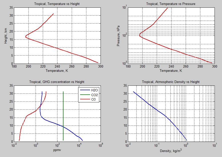
% ======== Plot standard atmosphere data if applicable
if std_atm>0

for i=1:nmol % create a legend for the GHGs on 3rd subplot
textleg2(i)={Hmols(mol(i),:)};
end

figure(5)
subplot(2,2,1),plot(Tinit,z/1000,’Linewidth’,2,’Color’,’Red’)
xlabel(‘Temperature, K’)
ylabel(‘Height, km’)
grid on
title([strtrim(AFGLname(std_atm,:)) ‘, Temperature vs Height’])

subplot(2,2,2),semilogy(Tinit,p/100,’Linewidth’,2,’Color’,’Red’)
set(gca,’YDir’,’reverse’)
xlabel(‘Temperature, K’)
ylabel(‘Pressure, hPa’)
grid on
title([strtrim(AFGLname(std_atm,:)) ‘, Temperature vs Pressure’])

subplot(2,2,3),semilogx(mix*1e6,z/1000,’Linewidth’,2)
xlabel(‘ppmv’)
grid on
title([strtrim(AFGLname(std_atm,:)) ‘, GHG concentration vs Height’])
legend(textleg2)

subplot(2,2,4),semilogx(rho,z/1000,’Linewidth’,2)
xlabel(‘Density, kg/m^3’)
grid on
title([strtrim(AFGLname(std_atm,:)) ‘, Atmospheric Density vs Height’])
end
end
% ==================================================

disp([‘—- End of Run —- ‘ datestr(now) ‘ —-‘]);

===== end of v 0.10.4======

===== Optical_3 ======

function [tau]=optical_3(vt, v, S, iso, gama, nair, molx, numz, numv, p, p0, Tlayer, T0,…
Na, rho, mair, dz, mol, nmol, mix, isoprop, contabs, linewon)

% Optical calculates tau as a function of wavenumber, v and layer,
% i=1-numz-1. Uses data read from the HITRAN database; p, T, rho from each
% layer; mol, mix, ison as the molecules with the mixing ratio and prescribed
% isotopes to consider

% v3 – minor change: mix is now a matrix mix(nmol,numz-1), i.e., mixing ratio for each
% molecule in each layer, & water vapor is now mix(1,1:numz-1), not mixh2o

c1=1.3515; c2=2.4371; c3=5.7216; a1=.8461; a2=0.4308; % coefficients for the
% approximation of transmission with spherical geometry
tau=zeros(numz-1,numv); % optical thickness
fprintf(‘%s’, ‘Calc optical thickness each layer.. ‘);
tau=zeros(numz-1,numv); % optical thickness matrix

% ———– Each layer ————————
for i=1:numz-1
fprintf(‘%d %s’, i, ‘ ‘); % display layer being calculated (this section takes the longest)

na=(Na*rho(i)/mair)/1e6; % number of air molecules per cm^3
d=100*dz(i); % path length in cm

% and so for this slab of depth, d:
% ———– Iterate through each GHG for this slab, m ————–
for m=1:nmol
% fprintf(‘%d %s’, m, ‘ ‘); % display molecule being calculated
if mol(m)==1 % if water vapor, special case
if contabs % if using continuum absorption
% method from Pierrehumbert 2010, p.260, uses svp & units
% in m2/kg

sig=continuum1000(vt,Tlayer(i)); % get capture cross section in m2/kg
% ** note non-std units ** and values are only valid for
% range defined in function continuum1000

% mixh2o = partial pressure of w.v. / pressure, so
% the partial pressure of water vapor = mixh2o(i) x p(i)
tau(i,:)=tau(i,:)+sig.*pi/100*(mix(m,i)*p(i))^2/(1e4*461.4.*Tlayer(i));
end
end
im=find(molx==mol(m)); % the index for all values of this GHG
immax=length(im); % the number of lines for this GHG
%disp([‘Layer ‘ num2str(i) ‘. Mixing ratio for molecule ‘ num2str(m) ‘ = ‘ num2str(mix(m))]);
% ——- Iterate through each absorption line for this GHG, j —-

for j=1:immax % each absorption line
% im(j) is the index for v, S, etc
% v(im(j))=line center, S(im(j))=line strength, gama(im(j))=half width
% now a code inefficient method – calculate the profile for each
% across the entire wavenumber range

% for this one line we need to find iso # and therefore the relevant
% proportion then x mixing ratio x no of air molecules
nummol=isoprop(m,iso(im(j)))*mix(m,i)*na;
% then calc the actual line width for this temp & pressure
if linewon % normal physics
ga=gama((im(j))).*(p(i)/p0).*(T0/Tlayer(i)).^nair((im(j)));
else % non-real physics for comparison
ga=gama(im(j));
end

% Pekka’s code improvement for v0.9.5
dt1=1./((vt-v(im(j))).^2+ga^2); % line shape across all wavenumbers
tau(i,:)=tau(i,:)+nummol*S(im(j))*ga*dt1; % change to tau for
% this layer and line for all wavenumbers
end % end of each absorption line, j
end % end of each GHG, m

tau(i,:)=d/pi*tau(i,:); % now include the 3 constants
% Zhao & Shi 2013 approximation (for spherical geometry)
r=1+1./tau(i,:).*log(1+tau(i,:)/2+tau(i,:)./(2*tau(i,:)+2+4.*(c1*tau(i,:).^a1+c2*tau(i,:))/(c3*tau(i,:).^a2+c2*tau(i,:)+1)));
tau(i,:)=r.*tau(i,:);
end % end of each layer, i
disp(‘ ‘);

end

===== end of Optical_3 ======

Related Articles

Part One – some background and basics

Part Two – some early results from a model with absorption and emission from basic physics and the HITRAN database

Part Three – Average Height of Emission – the complex subject of where the TOA radiation originated from, what is the “Average Height of Emission” and other questions

Part Four – Water Vapor – results of surface (downward) radiation and upward radiation at TOA as water vapor is changed

Part Six – Technical on Line Shapes – absorption lines get thineer as we move up through the atmosphere..

Part Seven – CO2 increases – changes to TOA in flux and spectrum as CO2 concentration is increased

Part Eight – CO2 Under Pressure – how the line width reduces (as we go up through the atmosphere) and what impact that has on CO2 increases

Part Nine – Reaching Equilibrium – when we start from some arbitrary point, how the climate model brings us back to equilibrium (for that case), and how the energy moves through the system

Part Ten – “Back Radiation” – calculations and expectations for surface radiation as CO2 is increased

Part Eleven – Stratospheric Cooling – why the stratosphere is expected to cool as CO2 increases

Part Twelve – Heating Rates – heating rate (‘C/day) for various levels in the atmosphere – especially useful for comparisons with other models.

References

The data used to create these graphs comes from the HITRAN database.

The HITRAN 2008 molecular spectroscopic database, by L.S. Rothman et al, Journal of Quantitative Spectroscopy & Radiative Transfer (2009)

The HITRAN 2004 molecular spectroscopic database, by L.S. Rothman et al., Journal of Quantitative Spectroscopy & Radiative Transfer (2005)

Read Full Post »

We’ve looked, via the model, at how radiation travels through, and interacts with, the atmosphere. But this has been for one set of atmospheric conditions which are listed in Part Two.

Water vapor is the most important atmospheric “greenhouse” gas.  But its effect on the surface radiation and TOA radiation are quite complex.

• Water vapor has absorption lines throughout most of the wavelengths of interest for terrestrial radiation (4-50 μm = 2500-200 cm^-1 )
• Whereas the CO2 concentration is “well-mixed”, i.e. broadly speaking the same mixing ratio or ppmv everywhere in the atmosphere, water vapor is concentrated much more in the lower atmosphere, especially in the planetary boundary layer – so the mixing ratio of water vapor might be 1000 times higher at the surface than at the top of the troposphere
• The water vapor continuum absorbs as a function of the square of the number of water vapor molecules – other gases like CO2 absorb as a linear function of the number of CO2 molecules

I ran the model described in Part Two many times, changing the boundary layer humidity (BLH), the free tropospheric humidity (FTH) and the surface temperature.

Boundary Layer Humidity

Here is how the TOA flux changes as the boundary layer humidity changes from 20-100% at free tropospheric humidity =60%:

Figure 1

Is this surprising?

Now the downward longwave radiation (DLR) at the surface with the same conditions:

Figure 2

I could plot some more comparisons with different FTH values, but regardless of the FTH value the graphs of TOA flux vs BLH have the same characteristics.

Why, if water vapor is such a strong GHG, does the top of atmosphere radiation stay almost the same for a boundary layer almost dry through to completely saturated?

The reason is simple. The surface is emitting a blackbody radiation spectrum for that surface temperature (see note 2 in Part Two). The boundary layer is at almost the same temperature as the surface (2-3K difference in this case) so at a given wavelength radiation either gets transmitted, or gets absorbed and re-emitted (usually a combination). But if re-emitted, it is at almost the same temperature as the surface.

The radiative transfer equations show us that the change in flux as radiation travels through a body is caused by the difference between the temperature of the source of the radiation and the temperature of the body in question. This is explained a little more in Part Two and is an essential point to grasp.

So the upward radiation at TOA is the almost the same whether the boundary layer is saturated or dry.

But the surface DLR experiences a big difference as the boundary layer moisture changes. The reason why should be obvious by now, but this subject is quite difficult to take in when you are new to it.

What downward radiation is incident on the boundary layer from above? The answer is – nothing like as much as is incident on the boundary layer from below. The downward atmospheric radiation on this boundary layer is just the emission from the various GHGs (water vapor, CO2, O3, etc) and the water vapor concentration above is quite a lot lower than the boundary layer.

When the boundary layer is saturated with water vapor it emits very strongly across many bands. So the humidity of the boundary layer has a big impact on the DLR, but very little on the TOA outgoing radiation.

Free Tropospheric Humidity

Now let’s see the TOA changes as free tropospheric humidity, FTH, is changed – with BLH fixed at 100%:

Figure 3

So now as the atmosphere above the boundary layer gets more water vapor it absorbs (and re-emits) more strongly. But the re-emission is from colder layers of the atmosphere so as this GHG increases in concentration up through the atmosphere, the TOA radiation reduces significantly. And if we reduce the outgoing radiation from the planet then, all other things being equal, the planet warms.

Let’s see the reasons a little more clearly, for the extreme case when we change FTH from 100% to 0%, with Ts=300K. The left side has the spectra for selected heights for both cases, and the right side has the difference between the two cases (at the same heights):

Figure 4 – Click to enlarge

[Note the title on the top right is slightly incorrect. It is not ΔTOA, it is the Δ (difference) at a few different heights including TOA.]

We can see that in the center of the CO2 band (600-700 cm^-1) there is zero change between the two cases at all heights – as expected.

The differences between the two cases occur:

• strongly around 200-550 cm^-1 (50-18 μm) where water vapor absorption is quite strong
• somewhat around the “atmospheric window” – which still absorbs due to the continuum, especially at the high water vapor saturation pressure when the surface temperature is near 300K
• strongly around the 1500 cm^-1 (7μm) region where there are lots of water vapor absorption lines – however the surface emission is not so high in the first place so the overall effect is reduced

Now let’s look at DLR at the surface:

Figure 5

Even though the boundary layer is saturated, changes in water vapor above this layer still have a significant impact on the surface DLR.

Let’s see why by comparing the spectra of the 100% and 0% cases at 300K:

Figure 6 – Click to enlarge

The dark blue curve is the one we are measuring at the surface. The top right is the difference between the two cases at four different heights. The bottom right shows only the difference in spectra at the surface (it is hard to see it in the top right graph).

What is clear is that the difference is caused by the “mid-strength” absorbing/emitting “atmospheric window around 800-1200 cm^-1. The “background” DLR from the very top of atmosphere is of course zero (see figure 6 in Part Two). So anything that adds to the DLR on the way down assists the surface spectra.

This is not the case for very strongly emitting regions – see the region around 500 cm^-1. The boundary layer emits and absorbs due to water vapor so strongly in this wavenumber region that incident radiation from above is irrelevant to the surface measurement.

With and Without Water Vapor

Now let’s look at the upward spectra at various heights with (saturated) and without (dry) water vapor:

Figure 7 – Click to enlarge

The bottom right graph is just the top layer in the top right graph shown separately for clarity.

Conclusion

Most people’s untrained intuition about how different radiatively-active gases (=”greenhouse” gases) in different concentrations at different locations change the interaction of radiation with the atmosphere are wrong. Intuition needs to be informed by measurement and theory. It’s just not an intuitive subject.

We’ve seen that water vapor can have very different effects on TOA radiation and the surface. And we’ve seen that water vapor in different places has very different effects. Also we’ve seen the difference between a dry and saturated atmosphere.

Three important points:

1. On a technical note – this model has at least one important flaw, which is to do with how absorption lines change near the top of the troposphere – the Voigt profile vs the Lorenzian profile.

The Voigt profile is not yet implemented because when I last looked at it it made my head hurt trying to implement it in a useful manner (my attempt at the Voigt profile turned a surprisingly fast model given the 287,000 lines calculated in each of 10 layers into a bucket of sludge).

I am going to have another crack at this headache-inducing puzzle before trying to do lots of “what happens when CO2 concentrations are changed by small amounts” scenarios.

Actually, if there are any maths whizzes out there who would like to do the heavy lifting – or even just explain what seems simple to someone who has forgotten almost all maths ever learnt – please let me know here or via email at scienceofdoom – the usual bit – gmail.com. Probably you will get your name on the top of one of the graphs or something, no promises on the font size yet.

2. These scenarios we have seen are all from a “snapshot” of the climate in 1D without running it to a new equilibrium. Obviously if you change the water vapor from 0% to 100% the surface temperature won’t stay the same. Everything will change. When we have been comparing scenarios we have had mostly the exact same surface and atmospheric temperature. This is for a good reason. Small steps first. Actually, grasping atmospheric radiative transfer is a big step.

3. Changes in water vapor affect not just radiative transfer but latent heat and convection. The deep convection that “cranks the engine” on the important tropical circulation is from solar heating over the warmest oceans (see Clouds & Water Vapor – Part Five – Back of the envelope calcs from Pierrehumbert). Radiative transfer is just one piece of the puzzle.

Related Articles

Part One – some background and basics

Part Two – some early results from a model with absorption and emission from basic physics and the HITRAN database

Part Three – Average Height of Emission – the complex subject of where the TOA radiation originated from, what is the “Average Height of Emission” and other questions

Part Five – The Code – code can be downloaded, includes some notes on each release

Part Six – Technical on Line Shapes – absorption lines get thineer as we move up through the atmosphere..

Part Seven – CO2 increases – changes to TOA in flux and spectrum as CO2 concentration is increased

Part Eight – CO2 Under Pressure – how the line width reduces (as we go up through the atmosphere) and what impact that has on CO2 increases

Part Nine – Reaching Equilibrium – when we start from some arbitrary point, how the climate model brings us back to equilibrium (for that case), and how the energy moves through the system

Part Ten – “Back Radiation” – calculations and expectations for surface radiation as CO2 is increased

Part Eleven – Stratospheric Cooling – why the stratosphere is expected to cool as CO2 increases

Part Twelve – Heating Rates – heating rate (‘C/day) for various levels in the atmosphere – especially useful for comparisons with other models.

References

The data used to create these graphs comes from the HITRAN database.

The HITRAN 2008 molecular spectroscopic database, by L.S. Rothman et al, Journal of Quantitative Spectroscopy & Radiative Transfer (2009)

The HITRAN 2004 molecular spectroscopic database, by L.S. Rothman et al., Journal of Quantitative Spectroscopy & Radiative Transfer (2005)

Read Full Post »

If you’ve just stumbled across this article without reading the earlier posts, please take a few minutes to review:

• Visualizing Atmospheric Radiation – Part One with a few basic concepts
• Part Two with some calculated spectra of upward radiation from the surface through to the top of atmosphere

Most people find the actual results of radiative transfer in the atmosphere non-intuitive. Intuition is not a good guide for this topic. So a lot of misconceptions arise because the results of atmospheric physics disagree with the mental models in people’s heads. Obviously the physics must be wrong or probably climate scientists haven’t understood the basics.. Shaking of heads.

For people interested in reality, read on.

We are still looking at how radiation travels and interacts with the atmosphere before anything changes.

There is a lot of fascination in the subject of the “average height of emission” of terrestrial radiation to space. If we take a very simple view, as the atmosphere gets more opaque to radiation (with more “greenhouse” gases) the emission to space must take place from a higher altitude. And higher altitudes are colder, so the magnitude of radiation emitted will be a lesser value. And so the earth emits less radiation and so warms up.

This “average height of emission” is often supplied as a mental model and it’s a good initial starting point.

Here is the result of the atmospheric model created with a surface temperature of 288K (15°C), 80% humidity in the boundary layer and 40% humidity above that (the “free troposphere). This is a cloud-free sample – clouds are very common, but really make life complicated and we are trying to provide a small level of enlightenment. Simple stuff first.

The model is the same as in Part Two – but with 20 layers instead of 10. More layers just means better resolution plus a little bit more accuracy. Each layer contains roughly the same number of molecules (same pressure differential between each layer), so each higher layer is progressively thicker.

The graph shows how much radiation (“flux”) makes it from the surface and from each atmospheric layer in the model to the top of the atmosphere (TOA) – [update Jan 9th, see revised graph in comments].

Figure 1

And here we’ve zoomed in by expanding the x-axis:

Figure 2

The TOA flux = 239.5 W/m², so what is the level where half of this value comes from below and half from above?

If we include the surface and the first 5 layers we don’t have quite half (48%), and if we go to 6 layers we get just over half (51%).  Layer 5 is centered at 1.9km with the top of this layer at 2.1km. Layer 6 is centered at 2.4km.

So let’s say the “average” height of emission to space is just over 2 km (in this example).

There’s probably a better mathematical way of expressing it (this is more like the “median height”) but in fact this “average emission height” is really a curiosity value number anyway. In the words of guru commenter Pekka Pirilä (on another topic):

Any number that is not observable and that’s not used as an input or intermediate value in any calculation that aims to produce observable results is of curiosity value only by definition.

So it’s interesting but you don’t find it a key subject of any climate science papers. Still, being as so many people find it fascinating we will see how it changes as “greenhouse” gases vary in concentration and temperature profiles change.

While we are looking at this, let’s see what wavenumbers from what levels make the largest contribution to the TOA flux. That is, let’s look at the spectral distribution vs height.

First the TOA spectra for these conditions (Ts=288K, Boundary layer humidity=80%, Free tropospheric humidity=40%):

Figure 3

Now to see where this all originated from we divide up the wavenumbers into bands of 100 cm^-1, and we see the contribution to the TOA flux by band and height in the atmosphere (note that height in km is now ‘lying on the side’ to the left and wavenumber to the right, lost the axes labels somewhere along the way):

Figure 4

Zooming in a little:

Figure 5

We see that in the “atmospheric window” between 800 cm^-1 to 1200 cm^-1 the surface transmits almost “straight through” (62% of surface flux makes it straight through to the top of atmosphere in this wavenumber range). A small component comes from around the center of the CO2 band (667 cm^-1) from the top layer. The rest mostly comes from the “wings” of the CO2 band and where the water vapor absorption is not so strong, around 400 cm^-1.

Conclusion

Hopefully seeing the actual data in these different ways helps to see that “average height of emission” is not a real concept or a particularly useful concept. Perhaps it’s a bit like averaging the kg of food consumed per day per person in the entire world. You get a value but the components that made it up are so wide ranging the average has lost anything useful. It’s not like average height of male 20-year olds in Latvia.

Transmission and emission of atmospheric radiation is extremely wavelength dependent.

Related Articles

Part One – some background and basics

Part Two – some early results from a model with absorption and emission from basic physics and the HITRAN database

Part Four – Water Vapor – results of surface (downward) radiation and upward radiation at TOA as water vapor is changed

Part Five – The Code – code can be downloaded, includes some notes on each release

Part Six – Technical on Line Shapes – absorption lines get thineer as we move up through the atmosphere..

Part Seven – CO2 increases – changes to TOA in flux and spectrum as CO2 concentration is increased

Part Eight – CO2 Under Pressure – how the line width reduces (as we go up through the atmosphere) and what impact that has on CO2 increases

Part Nine – Reaching Equilibrium – when we start from some arbitrary point, how the climate model brings us back to equilibrium (for that case), and how the energy moves through the system

Part Ten – “Back Radiation” – calculations and expectations for surface radiation as CO2 is increased

Part Eleven – Stratospheric Cooling – why the stratosphere is expected to cool as CO2 increases

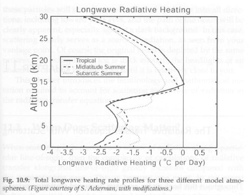
Part Twelve – Heating Rates – heating rate (‘C/day) for various levels in the atmosphere – especially useful for comparisons with other models.

References

The data used to create these graphs comes from the HITRAN database.

The HITRAN 2008 molecular spectroscopic database, by L.S. Rothman et al, Journal of Quantitative Spectroscopy & Radiative Transfer (2009)

The HITRAN 2004 molecular spectroscopic database, by L.S. Rothman et al., Journal of Quantitative Spectroscopy & Radiative Transfer (2005)

Read Full Post »