The Science of Doom

We reviewed some simple concepts in Part One.

I’ve created a MATLAB model which can do a reasonable job of calculating radiative transfer through the atmosphere. More details about the model to follow, but first let’s look at an actual result and the implications.

There are a whole set of starting conditions, some of which are:

• 10 layers (of roughly equal pressure change)
• surface temperature = 288K (15ºC)
• boundary layer humidity (BLH) = 80%, and boundary layer top of 920hPa
• free tropospheric humidity (FTH) = 40%
• lapse rate (the temperature profile in the atmosphere) = 6.5 K/km
• tropopause at 11.7km, isothermal atmosphere above at 212K and TOA at 50hPa

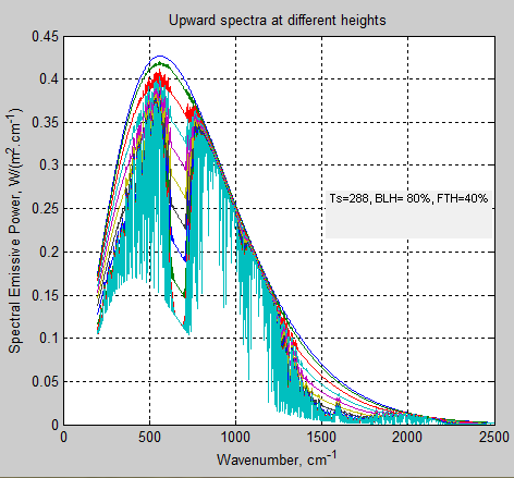
Figure 1

There’s a little too much information when we see all layers, so here are just four (see note 1):

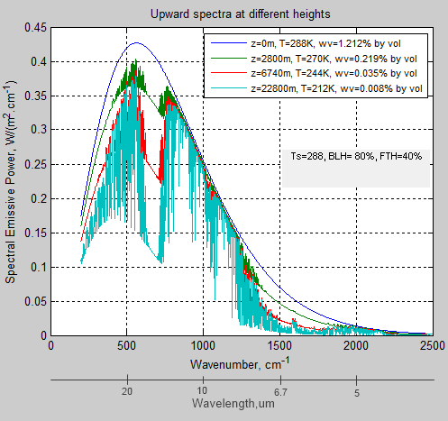
Figure 2 – Selected layers

What do we see?

Start at the top – the blue line – this is the emission of radiation upwards from the surface. In this case, for simplicity, the surface emissivity = 1.0 (see note 2) so this is the Planck function at 288K. The next curve down is at 2800m up where the temperature has dropped to 270K. The red curve is at 6740m & 244K, and the bottom curve is at 23km & 212K, well into the stratosphere.

Let’s zoom in on one region of wavenumbers/wavelengths:

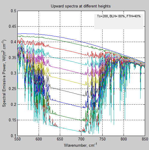
Figure 3 – Expanded view

First, the region 640-700 cm^-1 (14.3-15.6μm). The upward radiation at each higher altitude (which corresponds to each lower curve in the figure) is at the Planck blackbody function for the temperature of that layer.

The reason is that the incident radiation gets completely absorbed. Nothing gets out the other side. Transmissivity = 0, absorptivity = 1. It is “saturated”.

But we don’t see zero radiation. Why not?

The atmosphere is a strong absorber at these wavelengths, and therefore a strong emitter at these wavelengths. So each layer emits as a blackbody (in this region of wavelengths). We can easily see the temperature of the atmosphere from the Planck function if we are able to measure the radiation from these highly absorbing/emitting wavelengths.

Second, the region near 850 cm^-1 (below 12μm). See that the upward radiation at each altitude is almost at the surface radiation value. This is in the “atmospheric window” where the absorption is very low. The atmosphere is almost transparent at these wavelengths. So the absorption is low and the emission is low. But the starting point, if we can use that term, is the emission at the surface temperature of 288K. And so, in this wavelength region, at any point in the atmosphere the upwards radiation is close to the Planck curve of 288K. Basically, the intensity of radiation stays the same as it travels upward through the atmosphere because there is little absorption.

Transmitted Radiation Only

Just to make the subject of emission even clearer, here is a calculation where the atmosphere magically does not emit any radiation – compare this with figure 2:

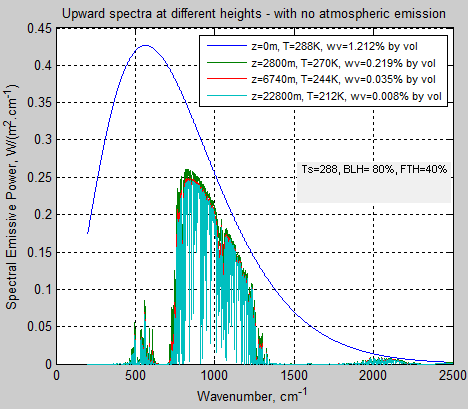
Figure 4 – No emission by the atmosphere

Even if we just look at the first 3 layers of the model (1.8km) we get pretty much the same view – i.e., most of the surface radiation is absorbed before we get very far through the atmosphere, but of course it is very wavelength dependent:

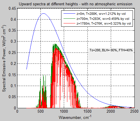
Figure 5 – No emission by the atmosphere

My calculation says that of 376 W/m² of surface emitted radiation between 200 cm^-1 and 2500 cm^-1, 75 W/m² (20%) gets transmitted to the top of atmosphere (note 4).

This is not all through the “atmospheric window” – you can see the wavelength dependence in figure 4. I calculate 61 W/m² through the atmospheric window (8-12μm), which means in that wavelength range 62% of surface radiation is being transmitted.

Up and Down Flux

Let’s look at the total (longwave) flux up and down through the atmosphere (note 3):

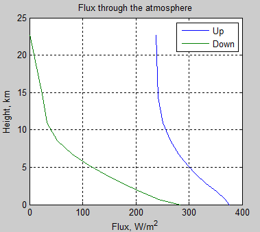
Figure 6

Notice that the downward flux is zero at the top of atmosphere. This is a boundary condition – there is no (significant) source of longwave radiation coming from outside the atmosphere. As we go down through the atmosphere it gets warmer and so the atmosphere emits more and more. Also as we go down the atmosphere there is much more water vapor, meaning the emissivity of the atmosphere increases significantly. So the atmosphere emits ever more radiation the closer we get to the surface.

We have already considered the upward transmission of radiation. Here the blue line on the graph is simply the sum (the “integral”) of the spectral components we saw in earlier graphs.

Why does the flux reduce with height? Because the absorption of upward radiation is greater than the emission of radiation upwards at each height.

If this point is not clear, please reread this article and Part One – if you are confused over this fundamental point it will be impossible to make good progress in understanding atmospheric radiation.

The absorptivity (the ability of the atmosphere to absorb radiation) is equal to the emissivity (the ability of the atmosphere to emit radiation) at any given wavelength. So why isn’t emission = absorption?

Because the incident upward radiation on a given layer comes from a higher temperature source:

• Absorption =incident radiation x absorptivity
• Emission = Planck function (blackbody radiation value) at the temperature of the gas x emissivity

Please ask if this is not crystal clear.

Net Flux & Heating or Cooling

If we want to do any heat transfer calculations we need to look at how the flux changes through the atmosphere. How much radiation enters and how much leaves (see note 5). Anything different from zero for a given layer means there must be heating or cooling by radiation. (This could be balanced by convection – and by absorbed solar radiation).

Let’s see the flux changes for each layer:

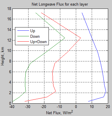
Figure 7

What this is showing is the calculation of (radiation in – radiation out) for each layer. As should be obvious from the previous figure, the upward path of longwave radiation is heating the atmosphere (more is absorbed than is emitted), whereas the downward path of longwave radiation is cooling the atmosphere (more is emitted than is absorbed).

When we sum both up we find that the atmosphere is cooling via radiation. “Greenhouse” gases are cooling the atmosphere! If only climate science considered the basics!

Each of the layers in the model contains a similar number of molecules – this is because I divided the atmosphere up into approximately equal pressure sections. This means that 10 W/m² cooling in any layer should equate to similar temperature changes in each layer, but let’s do that calculation anyway (heating rate per unit area/[specific heat capacity x density x depth of layer]):

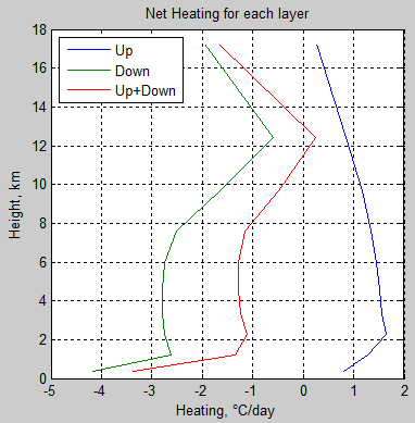
Figure 8 – Heating (cooling) from longwave radiation

The atmosphere is not actually transparent to solar radiation and you can find similar graphs of Net Shortwave Heating per Day in many climate science textbooks and papers.  The humid lower atmosphere gets a strong solar heating via water vapor. See Atmospheric Radiation and the “Greenhouse” Effect – Part Eleven – Heating Rates.

My graph doesn’t actually reproduce the magnitude of the cooling rates seen for standard atmospheres – typically around 2°C/day in the lower atmosphere but I’m pleased with getting the profile quite similar – remember that the “divergence” is the difference between two values. In this case, the up and down fluxes are in the 200-400 W/m² range, while the net is around 10-20 W/m².

To see what actual difference there is from a more complete model we would need to plug in one of the “standard atmospheres” and compare. The exact profile of water vapor concentration and atmospheric temperature have a big effect – something we will be looking at in detail anyway in later articles.

Convection

The calculation of radiative transfer in the atmosphere can be done for a given profile without knowing anything about convection. That is, if we know where we are right now – without knowing how we got here – we can still do an accurate calculation of how energy moves through the atmosphere by radiation.

If we want to predict the result of how the radiative heating/cooling changes the surface and atmospheric temperature then of course we need a model of convection – and atmospheric circulation.

Conclusion

What the model has done so far is taken:

• a given temperature profile
• a given concentration of GHGs including water vapor
• the large spectroscopic database of absorption lines complied by professionals over decades

– and used basic theory well-known and proven for many decades to calculate the upward and downward path of radiation through the atmosphere.

There’s lots to consider further. But the points and subjects in this article are all fundamental to understanding atmospheric radiation. So if anything is not clear, please ask questions.

Related Articles

Part One – some background and basics

Part Two – some early results from a model with absorption and emission from basic physics and the HITRAN database

Part Three – Average Height of Emission – the complex subject of where the TOA radiation originated from, what is the “Average Height of Emission” and other questions

Part Four – Water Vapor – results of surface (downward) radiation and upward radiation at TOA as water vapor is changed

Part Five – The Code – code can be downloaded, includes some notes on each release

Part Six – Technical on Line Shapes – absorption lines get thineer as we move up through the atmosphere..

Part Seven – CO2 increases – changes to TOA in flux and spectrum as CO2 concentration is increased

Part Eight – CO2 Under Pressure – how the line width reduces (as we go up through the atmosphere) and what impact that has on CO2 increases

Part Nine – Reaching Equilibrium – when we start from some arbitrary point, how the climate model brings us back to equilibrium (for that case), and how the energy moves through the system

Part Ten – “Back Radiation” – calculations and expectations for surface radiation as CO2 is increased

Part Eleven – Stratospheric Cooling – why the stratosphere is expected to cool as CO2 increases

Part Twelve – Heating Rates – heating rate (‘C/day) for various levels in the atmosphere – especially useful for comparisons with other models.

 

References

The data used to create these graphs comes from the HITRAN database.

The HITRAN 2008 molecular spectroscopic database, by L.S. Rothman et al, Journal of Quantitative Spectroscopy & Radiative Transfer (2009)

The HITRAN 2004 molecular spectroscopic database, by L.S. Rothman et al., Journal of Quantitative Spectroscopy & Radiative Transfer (2005)

Notes

Note 1: There is a slight inconsistency in the data presentation. There are 11 boundaries and therefore 10 layers. The spectra are calculated at the boundaries. The water vapor mixing ratio is calculated in the middle of the layer.

The calculation of emission of radiation is based on the temperature and the concentration of each GHG, including water vapor, in the mid-layer (the mid-pressure point in each layer) .

Note 2: The surface emissivity for the ocean, for example, is about 0.96 – see Emissivity of the Ocean. In some parts of the blogworld assuming an emissivity of 1.0 is a heresy that demonstrates what these inappropriately-named “skeptics” have known all along, climate science assumes an “unphysical blackbody model of the world”! And therefore cannot be taken seriously. More exclamation marks and so on.

I could have set an emissivity of 0.96 for the surface and this would have reduced the emitted upward radiation from the surface by 4%. But then for a radiative transfer calculation I would need to reflect 4% of the downward atmospheric radiation upwards (what is not absorbed or transmitted must be reflected). So in fact the upward radiation difference for the two cases (emissivity of 1.0 and 0.96) is quite small, less than 1% and not particularly useful for this calculation.

Note 3: Climate science uses the conventions of shortwave and longwave radiation. Shortwave is wavelengths less than 4μm (wavenumbers greater than 2500cm^-1), while longwave is greater than 4μm.

99% of solar radiation is shortwave, while 99% of all terrestrial radiation is longwave. This makes it easy to separate the two. See The Sun and Max Planck Agree – Part Two.

Note 4: The emission of thermal radiation by a surface at 288K with an emissivity of 1.0 is 390 W/m². This is across all wavelengths. The model looks at the range of wavenumbers that equates to 4-50μm to ease up the calculation effort required. Almost all of the “missing spectrum” is in the far infra-red (longer wavelengths/lower wavenumbers), and is subject to relatively high absorption from water vapor.

Note 5: If you hear the technical term flux divergence it is essentially the same thing. Flux divergence is per unit volume so it isn’t such a useful value. Instead the most common term is heating rate which divides the gain (loss) in radiation energy by the heat capacity to calculate the radiative heating (cooling) rate per unit of time (typically per day).

Read Full Post »