In Part Nine – Data I – Ts vs OLR we looked at the monthly surface temperature (“skin temperature”) from NCAR vs OLR measured by CERES. The slope of the data was about 2 W/m² per 1K surface temperature change. Commentators pointed out that this was really the seasonal relationship – it probably didn’t indicate anything further.
In Part Ten we looked at anomaly data: first where monthly means were removed; and then where daily means were removed. Mostly the data appeared to be a big noisy scatter plot with no slope. The main reason that I could see for this lack of relationship was that anomaly data didn’t “keep going” in one direction for more than a few days. So it’s perhaps unreasonable to expect that we would find any relationship, given that most circulation changes take time.
We haven’t yet looked at regional versions of Ts vs OLR, the main reason is I can’t yet see what we can usefully plot. A large amount of heat is exported from the tropics to the poles and so without being able to itemize the amount of heat lost from a tropical region or the amount of heat gained by a mid-latitude or polar region, what could we deduce? One solution is to look at the whole globe in totality – which is what we have done.
In this article we’ll look at the mean global annual data. We only have CERES data for complete years from 2001 to 2013 (data wasn’t available to end of the 2014 when I downloaded it).
Here are the time-series plots for surface temperature and OLR:
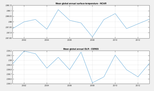
Figure 1
Here is the scatter plot of the above data, along with the best-fit linear interpolation:
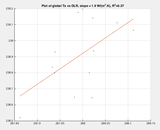
Figure 2
The calculated slope is similar to the results we obtained from the monthly data (which probably showed the seasonal relationship). This is definitely the year to year data, but also gives us a slope that indicates positive feedback. The correlation is not strong, as indicated by the R² value of 0.37, but it exists.
As explained in previous posts, a change of 3.6 W/m² per 1K is a “no feedback” relationship, where a uniform 1K change in surface & atmospheric temperature causes an OLR increase of 3.6 W/m² due to increased surface and atmospheric radiation – a greater increase in OLR would be negative feedback and a smaller increase would be positive feedback (e.g. see Part Eight with the plot of OLR changes vs latitude and height, which integrated globally gives 3.6 W/m²).
The problem of the”no feedback” calculation is perhaps a bit more complicated and I want to dig into this calculation at some stage.
I haven’t looked at whether the result is sensitive to the date of the start of year. Next, I want to look at the changes in humidity, especially upper tropospheric water vapor, which is a key area for radiative changes. This will be a bit of work, because AIRS data comes in big files (there is a lot of data).


SOD,
You wrote: “The correlation is not strong, as indicated by the R² value of 0.37, but it exists.”
Could you explain what you mean by “it exists”? That it passes a some significance test at a particular level?
Frankly, I don’t see any correlation.
No, I don’t have any confidence in significance tests for this kind of relationship. I simply mean there is measured correlation – that’s all.
Significance tests – i.e. some probability attached, or null hypothesis at a particular confidence interval – rely on a theory about the relationship between the data points.
That’s what an R2 calculation tells you. It tells you there is one. It is the percentage of the OLR variation that is explained by a linear model. With 13 datapoints I don’t see what else can be usefully produced (other than a linear fit).
This also means that 63% is not explained by the linear relationship. It also means, with 13 datapoints, that the results are sensitive to some values.
I leave the statistical runes to others, given my general skepticism about statistical intepretation for complex non-linear dynamic systems.
SOD,
“given my general skepticism about statistical intepretation for complex non-linear dynamic systems.”
I second that. But I suspect that even with a linear system with random, independent errors, an R^2 of 0.37 with 13 points could be random chance.
SOD,
Just tried plotting the data myself. When I fit OLR vs. T, I got the same slope as you (1.9), borderline significant at 95% level using the usual linear regression assumptions. When I fit T vs. OLR, I got a borderline significant inverse slope of 6.2. I have forgotten what it is called when you get such different results depending on which variable is taken as independent but I have not forgotten what it means. You can’t trust the result unless you know that errors in one variable are insignificant and you use that variable as the independent one. I doubt that is true for T here.
I am disappointed to see this, since I think your site is generally grade A quality.
Mike M
I will be happy to see others produce interpretations of the data. The motivation for producing these articles analyzing the data myself was the question by a commenter on Part Eight – Clear Sky Comparison of Models with ERBE and CERES:
– so I promised to attempt to reproduce some data so we could assess questions like this.
If the graph had a slope that showed 4.0 W/m2 – i.e., negative feedback of the climate system – with an R2 statistic of 0.37 and I didn’t publish the results because the correlation was weak I suspect many people would equally question my decision and also be disappointed. Luckily I don’t care about people’s disappointment.
Another approach to data analysis of these 13 points suggested by readers will be invaluable.
My statistical prowess is limited to calculating means, variances, R2 and the like – and to only calculating statistical significance of data that meets the criteria of independent and identically distributed random variables.
I can also do a party piece with significance of simple autocorrelated data but that presupposes we believe the test that clarifies this relationship – and mostly climate data isn’t a nice fit to a simple first order autocorrelation.
At some point I would like to take some non-linear dynamic systems and demonstrate the futility of calculations of statistical significance – or maybe prove my own working hypothesis wrong. But that’s another story.
I noticed that Roy Spencer has an article about 15 years of OLR data. The CERES data started March 2000 and the March 2015 data is apparently just out.
I’d like at some point to see whether the results I got are the same – for example, extending the results here from March 2000 (instead of January 2001) to March 2015 instead of to December 2013.
When I downloaded the data, once of the datasets (AIRS, CERES, NCAR) was only available to late 2014 (not to December 2014).
But for now, just a note for people who have taken a cursory look at this article and his article – the measurement he is looking at is a more complete one – net radiation.
We are looking here at changes in OLR – which tells us about changes in emission of terrestrial radiation. “Net radiation” = changes in OLR plus changes in reflected solar, i.e. also includes changes in (primarily) cloud reflectivity.
Another two notes:
1. As already stated in earlier parts of this series (and originally covered in Measuring Climate Sensitivity – Part One) – there is a problem with compounding cause and effect, where the OLR changes resulting from temperature changes are not independent of radiation fluctuations causing temperature changes that go on to affect OLR.
2. The idea that the climate has an invariant climate sensitivity is a simple idea that is very likely wrong. Only the crushing disappointment of trying to deal with that idea and not being able to measure anything useful about climate sensitivity has motivated people to work from an “ideal” standpoint and not think too much about the problem that climate sensitivity is probably a function of time and climate state..
From time to time I have thought that attempting to measure climate sensitivity was a hopeless case. Still it’s interesting to pull the results out and see what they might show us under some limiting conditions.
You could use Total Least Squares to fit a linear model. That takes the errors in both variables into account. Trying to do something about serial autocorrelation with only 13 noisy data points is a non-starter.
I suspect the point in the lower left corner of the graph has a strong effect on the slope and the value of R².
My instinct told me that this data means nothing about climate, then when I eyeballed the time series plots and get (0.1W/m2)/(0.05K)= 2.0. Maybe it is reasonable. Dewitt is right, the scatter plot result looks like it is controlled by the lower left data point. All in all, being 40% confident that such a relationship may actually exists does seem to make sense.
This is (I assume 3.7/2.0) a TCS of 1.85K, which seems reasonable.
Spenser lags OLR 4 months to “maximize correlation” and gets a TCS of 1.3 (which matches his climate box model). Would that lag change account for a 0.5K TCS difference? He is also getting an R2 of 0.57, which sounds better, but is that just due to his 4-month lag?
The other interesting point for me is that both the SOD and Spenser plots are within the dreaded Pause. Does this mean that these “pause” TCS estimates are biased low?
Now, I am back to my original instinct that the ~15-year time-frame is too short to draw any real conclusion.
Howard,
You wrote: “This is (I assume 3.7/2.0) a TCS of 1.85K, which seems reasonable.”
Your logic is right, but since this is an estimate based on energy balance, it would be an ECS of 1.85 K
“Spenser … gets a TCS of 1.3”.
He does not seem to say if his latest estimate is TCS or ECS, but he says it is the same as his previous estimate, which was ECS.
“The other interesting point for me is that both the SOD and Spenser plots are within the dreaded Pause. Does this mean that these “pause” TCS estimates are biased low?”
Not necessarily. The beauty of this method (if it is valid) is that it does not really matter if the variation is internal or external.
“Now, I am back to my original instinct that the ~15-year time-frame is too short to draw any real conclusion.”
That is certainly true for methods based on trends in global T or ocean heat content. But for this method the time frame should not matter. What does matter is getting enough data points for reasonable statistics. That might be accomplished by appropriate disaggregation of the data. That appears to work for clear sky conditions (part nine, I think) but looks dicey when there are clouds.
Mike M: 15-years seems impossibly short to get an ECS. Also, getting reasonable stats might just be measuring a minor limb of an insignificant peak on the flank of a great mountain.
As far as the internal or external cause, it does matter because the relationship is not OLR=kT, it’s more like OLR = kT +/- (a bunch of other first-order feedback factors). Maybe some years or decades, positive feedbacks dominate, then fade and negative feedbacks dominate for some time. For instance, lets assume the Iris effect is real, but it waxes and wanes based on the AMO cycle.
Howard,
“15-years seems impossibly short to get an ECS.”
From trends, yes. But I don’t see how one can make a blanket statement of that type.
“the relationship is not OLR=kT, it’s more like OLR = kT +/- (a bunch of other first-order feedback factors)”
The relation is OLR = kT where kT includes all the first order feedback factors. So by definition there are no other first order feedback factors. There might well be other non-feedback causes of variation in OLR that might plausibly appear as noise.
The idea that feedbacks might not be constant is intriguing, but strictly speaking I think that such feedbacks would have to be other than first order. But I suppose they could appear to be first order in T while also depending on something else (bilinear behavior, for example).
“For instance, lets assume the Iris effect is real, but it waxes and wanes based on the AMO cycle.”
Without a physically plausible model for such effects, they are just speculation. I do not think that such speculation would constitute a valid criticism of an attempt to estimate sensitivity. But they would constitute a reason to be cautious about using the estimate to extrapolate over long time scales.
“15-years seems impossibly short to get an ECS.”
From trends, yes. But I don’t see how one can make a blanket statement of that type.
To my mind, ECS is a theoretical asymptote that is never reached. Looking at the Pleistocene paleo data, it seems like temperature declines ever downward punctuated by transient reversals until the ice sheets catastrophically fail. I don’t see any evidence of equilibrium.
“the relationship is not OLR=kT, it’s more like OLR = kT +/- (a bunch of other first-order feedback factors)”
The relation is OLR = kT where kT includes all the first order feedback factors. So by definition there are no other first order feedback factors. There might well be other non-feedback causes of variation in OLR that might plausibly appear as noise.
It seems a little simplistic to lump first order feedbacks into a single proportionality constant.
The idea that feedbacks might not be constant is intriguing, but strictly speaking I think that such feedbacks would have to be other than first order. But I suppose they could appear to be first order in T while also depending on something else (bilinear behavior, for example).
How long will it take for the Arctic sea ice to become ice free. How long will it take to melt the dreaded methane clathrates? How long before the ice sheet meltwater and associated sediment causes ocean circulation changes? Maybe none of this matters, but we don’t know enough
“For instance, lets assume the Iris effect is real, but it waxes and wanes based on the AMO cycle.”
Without a physically plausible model for such effects, they are just speculation. I do not think that such speculation would constitute a valid criticism of an attempt to estimate sensitivity. But they would constitute a reason to be cautious about using the estimate to extrapolate over long time scales.
Absolute speculation…. however, so are the current crop of GCMs. Thats what makes climate so interesting. The physics, biology and chemistry is pretty well understood on the granular level, it’s the 1,000-year, 30,000-foot view that remains a mystery.
Howard,
I agree with almost everything you say here. The exception is: “It seems a little simplistic to lump first order feedbacks into a single proportionality constant”.
It is, of course important to understand all the individual feedbacks. But it is also important to understand the net effect of all the feedbacks for the climate system as it presently exists. That is, I think, the limited but important question that SoD is attempting to address here. Determining that lumped together number serves two purposes: it gives us a first order estimate of how the climate might respond to increased CO2 and it gives us a check on the individual feedbacks.
I would say that natural variation on every time scale from a few decades on up remains pretty much a mystery. It is a shame that the modellers have given that short shrift.
Determining that lumped together number serves two purposes: it gives us a first order estimate of how the climate might respond to increased CO2 and it gives us a check on the individual feedbacks.
Exactly right. The simple analytical model is quite useful. ..especially since an accurate complex model is likely unachievable.
SOD: Earlier (less reliable?) OLR data from ERBE exists and I think there is at least one OLR composite record that has been put together from multiple sources in the satellite era. More quality data would certainly help.
http://olr.umd.edu
Mauritzen and Stevens (2015): Missing iris effect as a possible cause of muted hydrological change and high climate sensitivity in models, has a nice graph (Fig. 2) comparing observed (CERES-EBAF) and CMIP5 model regression results for SW, LW and net radaition over 2001-2013. Unfortunately it is for the tropics (20S-20N), not global. Monthly mean de-seasonalised anomalies are used. One can preview the graph at reduced resolution here: http://www.nature.com/ngeo/journal/v8/n5/full/ngeo2414.html
The graph shows that almost all CMIP5 models have a significantly lower response of OLR to surface temperature than shown by the observations. The observed increase is just over 4 W/m2/K. That is greater than the Planck response, notwithstanding that LW water vapour (WV) feedback should be highest in the tropics (1.8 W/m2/K at constant relative humidity). There is however a positive (albeit rather smaller than in most CMIP5 models) SW feedback of ~0.9 W/m2/K, which will include non-negligible SW absorption by increased WV as well as SW cloud feedback.
Since the title of this series is “Clouds and Water Vapor,” would it be possible to normalize the OLR data with respect to humidity before correlating it to temperature? Perhaps this is what you already have in mind. OLR directly reflects the combined influence of humidity and temperature. Clouds may still confound, but lag time effects may emerge due to this normalization.
More importantly, I am troubled by the definition of “no feedback” and look forward to your addressing this in future. The data is showing a linear relationship of about 2 W/m2/degK supposedly resulting from a theoretical 3.6 – 1.6 by compensating for humidity. If that hypothesis is correct, some type of normalization should move the slope toward 3.6 and improve the R squared.
An alternative to normalizing would be to segregate the data into more humid vs. less humid time intervals.
Chic,
We’ll be having a look at humidity data shortly. But you can’t “normalize it” to OLR easily. There is a strongly non-linear response of OLR to humidity – dependent on concentration and height, as well as what is below that level.
For example, add a few g/kg of water vapor over a very dry region and you get a totally different OLR response from that over a tropical wet region. Add x g/kg at 300mbar and you get a different OLR response from x g/kg at 600mbar. And so on.
Take a look at Clouds & Water Vapor – Part Six – Nonlinearity and Dry Atmospheres.
No type of normalization will move the slope to a linear relationship unless the global annual mean climate always responds exactly the same way to the same temperature perturbation.
Of course it won’t be easy, that’s why I proposed it instead of trying it myself.
I need to explain my reasoning on the second part. The OLR vs. surface temperature data is already linear to a degree at 2 W/m2/degK. If normalization or segregation was feasible whereby the influence of humidity and temperature were separated, and the 1.6 W/m2/degK signal was removed, then the slope might be closer to 3.6. Mute point if normalization is problematic.
There is some discussion at WUWT today with some bearing on this topic. I’ll explain later.
Note comments before and after.
The comment at WUWT gives a formula for the Planck response = 4*e*sigma*T^3 which is 3.6 W/m2/degK if e=0.96 and T=255 or if e=0.665 and T=288. Why do you use 3.6 W/m2/degK as the no feedback reference point for a regression of OLR vs. surface temperature considering that most OLR originates from the middle and upper troposphere?
One of the key points in the discussion is the non-linearity of the emissivity of water vapor. There is also an argument over a maximum possible emitting temperature of CO2 being 193K. The latter is off-topic, but the former relates to this post. Any thoughts?
Chic,
That formula is the change in emitted power from the surface with respect to change in surface temperature.
The calculation that produces 3.6 W/m2 per 1K surface and atmosphere temperature change – i.e., the “no feedback” response – is not calculated from that formula.
Here’s an example, shown in Part Eight – Clear Sky Comparison of Models with ERBE and CERES of the actual calculation:
Basically, change the surface and atmospheric temperature by 1K uniformly and calculate the change in OLR at the top of atmosphere at each latitude using the radiative-transfer equations. Then integrate the results to work out the global OLR response.
I had a very brief look at the discussion you highlighted. It would take a lot of time to explain all the flaws in the confused ideas of WUWT commenters so my best recommendation is to read a few textbooks instead of reading comments at WUWT and you will be much better off.
Is it this statement that you are asking about?
It’s a mishmash of technical words.
A black body at 193K has peak energy at wavelength = 15 μm. That’s just the shape of the radiance vs wavelength curve – the peak moves towards longer wavelengths as it gets colder.
Radiatively-active molecules in the atmosphere (let’s call them them “GHGs” for short) emit at some wavelengths and not others. In the center of the 15 μm band, CO2 emits and absorbs like a blackbody – i.e. its emissivity at that wavelength = 1 – with anything like atmospheric concentrations of GHGs.
For example, at the surface 95% of radiation at “exactly” 15 μm is absorbed within 1m of the atmosphere.
Think of the emissivity of CO2 being a function of wavelength. We would write this ε(λ). ε(λ=15) = 1, ε(λ=10) = 0. And at other wavelengths the emissivity is a value between 0 and 1.
Back to the “black body emitter”, as you change the temperature of a black body the peak wavelength moves. At hotter temperatures the peak wavelength is shorter. But the intensity of a hotter body at a given wavelength is always higher than the intensity of a colder body.
Here is a graph of some blackbody curves from 190K to 310K. You can see that the 15 μm intensity is greater at 310K than at 190K.
Chic: I made some comments on the WUWT post. They may be useful. (I hope SOD’s critical remarks didn’t apply to mine. He has been very generous in straightening out some of my misunderstandings.)
It may help to think about the difference between emission and emissivity. Let’s look at the emission term (the first term) of the Schwarzschild equation for radiation moving through and atmosphere (or any medium):
dI = n*o*B(lambda,T)*dz – n*o*I_0*dz
where n is the concentration of the GHG, o is the absorption cross-section, B(lambda,T) is the Planck function and dI is the amount of radiation added – emission – by the GHG found between altitude Z to Z+dz. Emission depends on how many GHG molecules are present and their absorption cross-section.
Now let’s look at emissivity for a single wavelength, the ratio of emitted radiation to blackbody radiation.
e = I/B(lambda,T)
What happened to the dependence on the amount of GHG and cross-section? Why is emissivity a constant independent of these two factors while emission depends on them?
Emissivity assumes that absorption and emission in the Schwarzschild equation have come into equilibrium with each other, so that dI is zero and I_0 = B(lambda,T). Everything having to do with black- and graybody radiation assumes that absorption and emission have come into equilibrium. The derivation of the Planck eqn assumes such an equilibrium.
When you try to apply concepts from blackbody radiation to the atmosphere, you run into the problem that such an equilibrium exists at only some wavelengths and for some altitudes. Since T changes with altitude, so does B(lambda,T) and I_0 at equilibrium.
People talk about an optically-thick layer of atmosphere – meaning that it emits blackbody or possibly graybody radiation. They also discuss an optically thin layer – meaning it emits proportionally to n*o. SOD has referred to n*o as the emissivity of an optically thin layer. Emissivity can be a very misleading concept to use when discussing the atmosphere. Yes, you can pretend the whole planet is a blackbox. However, OLR reaching space is emitted from places with very different temperature. What is the “right” temperature to use?
Frank
No, they didn’t apply to your comments.
So the spectral intensity of CO2 at 15 μm for atmospheric concentrations at 290K is 5.9x the spectral intensity at 190K:
18.7/3.2 = 5.9.
scienceofdoom and Frank,
Your comments are much appreciated. I definitely understand the reasons for much confusion on these concepts. I’m beginning to understand the particulars of CO2 absorption and emission better.
The commenter who you quote above and that Frank engaged with at WUWT is arguing that CO2 is not a black body and therefore CO2 at 290K cannot emit radiation at 5.9x the spectral intensity that it would emit at 193K. I assume his argument is based on quantum chemistry which I have not studied since college a long time ago. My interpretation of his argument is that 193K is a minimum temperature for CO2 to emit anything at all and that, at greater temperatures, the energy of the 15u emission is what it is. IOW, being at a greater temperature does not make the 15u photon any more intense.
This is just my interpretation and I plan to get it corrected or affirmed.
Chic,
CO2 is not a black body emitter across the entire spectrum. At 15 μm CO2 has an emissivity of 1 (with atmospheric concentrations of CO2). This means it is like a black body at certain wavelengths.
When you look up from the surface here you see that CO2 has a much higher radiance at 15 μm (wavenumber = 667 cm-1) than when you look down from 20km.
(The curves super-imposed are black body curves at different temperatures).
The surface in this polar region is at a higher temperature than the atmosphere at an altitude of 20km.
This graph is easily explained by the theory as found in physics textbooks. It is not easily explained by people who don’t understand emission and absorption of thermal radiation by GHGs.
You can see more measurements at Understanding Atmospheric Radiation and the “Greenhouse” Effect – Part Ten.
CO2 molecules will emit 15μm radiation as long as there is sufficient kinetic energy, i.e. the temperature is high enough, that a non-zero fraction is in the excited state. That temperature is a lot lower than 193K. The intensity of the radiation is proportional to the number of molecules in the excited state. That number increases with increasing temperature. The fact that the energy of a 15μm photon doesn’t change is not relevant.
You can calculate the fraction in the excited state using the Boltzmann Distribution:
f(E)=Aexp(-E/kT)
where E is the energy of the excited state, A is the degeneracy, i.e. the number of identical energy levels for that state, k is the Boltzmann constant and T is the temperature. For CO2 at 15μm, E is 7.9751kJ/mole and A is 2. So at 193K, the fraction in the excited state is ~0.014. At 100K, it’s ~0.00014. So even at 100K, there would be some emission.
If you want to play, an energy, wavelength, frequency converter is here.
A fractional population calculator is here.
The reason A=2 for CO2 is that the 15μm state for CO2 is a bending vibration and you can have two orthogonal states, referred to as in plane and out of plane. See here for more information on molecular vibrational modes.
That helps. So the intensity is a function of the wavelength, the concentration, and the fraction of the concentration in the excited state, which is determined by the temperature.
Chic,
To sum up, each of the Planck curves shown above are the black body emission values at different wavelengths. Each curve is a different temperature.
Nothing can ever radiate more than the black body curve.
[The fact that a gas is not a black body doesn’t mean it doesn’t radiate as strongly as a black body at some wavelengths. Many people who have “learnt” their radiative physics by reading blogs get the two ideas confused.]
The emissivity of gases is a very strong function of wavelength. The HITRAN database contains measurements, at each wavelength, of an absorption/emission parameter – usually written as σλ. (The subscript λ shows it is a function of wavelength).
The calculation of emissivity is actually very simple.
How many molecules, n, in the path (i.e. through the layer of atmosphere being considered) per unit area? Multiply by the absorption/emission parameter. The result is optical thickness: τλ = nσλ.
The emissivity, ελ = 1 – exp(-τλ).
Not being sure of your maths, and not wanting to either talk down to you or scare you off with formulas:
– if τ = 0, that is, there is no absorption/emission at this wavelength, then ε = 0
– if τ = 10, that is, there is very strong absorption/emission at this wavelength, then ε = 1.000
Then the radiance at a given wavelength is the Planck value at that wavelength (=blackbody value) x ε.
There’s nothing controversial about any of this. Not in textbooks.
No thermal source rather than nothing. Non-thermal sources, like lasers and microwave ovens, can have radiative intensities over a narrow wavelength band that are much, much higher than the temperature of the laser or the microwave cavity. A laser works, in fact, by creating a population inversion, where the fraction in the excited state is much higher than the thermal fraction. Then, if the configuration is correct, stimulated, rather than spontaneous, emission becomes dominant and all the excited states decay at once by photon emission.
Chic: I’m not sure where Hockeyschtick comes up with the claim that CO2 can’t emit more than a blackbody at 193 K. (I tried looking, but got disgusted with some distortions I read and gave up in disgust.)
An optically thick layer of GHG emits B(lambda,T) at any wavelength. An optically thin layer of GHG of height h emits h*n*o*B(lambda,T) – if we ignore the photons absorbed by the layer before they exit. So emissivity from a layer of GHG at any wavelength ranges from 1 at the upper limit to less than h*n*o at a lower limit and needs to be integrated over all wavelengths. I don’t see how this mathematics can yield a maximum emissivity or blackbody temperature for CO2. With a large enough n or h, h*n*o eventually approaches 1 unless o = 0.
I went to the online MODTRAN calculator and tried looking up from the ground through a US Standard atmosphere with only CO2 – 100, 200, 400, 800, 1600 ppm. 400 ppm was 85.5 W/m2 (blackbody equivalent 197 K) and each doubling was worth 6.5 W/m2 (about 4 K). So the emissivity of CO2 in our atmosphere is about 0.22 assuming T = 288 and it changes about 0.016 for every doubling. With 999999 ppm of CO2, the downward flux reaches 218 W/m2 (blackbody equivalent 249 K, emissivity 0.56). In some sense, this might be the maximum emissivity of CO2 at 1 atmosphere.
Interestingly, if I remove all CO2, there is still 24 W/m2 of DLR with a maximum about 8 um. If I remember correctly O2 has some weak lines.
Frank,
You can’t zero out the CFC’s or CO in MODTRAN. That’s probably where all the residual atmospheric emission is coming from.
Frank,
You raise many issues here in addition to Hockeyschtick’s interpretation of CO2 maximum emission at 15micron/193K. Sounded like he contradicted himself at times. And I’m sure he would not agree that an optically thick layer of pure CO2 would emit B(lambda,T) at any wavelength. Would you? Hockeystick is approaching the subject from the point of view that CO2 molecules are not black bodies and therefore the Planck function isn’t applicable. This is where I think he is contradictory, because he gets the max 193K from Wein’s Law which follows from the derivative of the Planck function, doesn’t it?
I’m taking the conservative position that follows from the textbook principles outlined by scienceofdoom and DeWitt Payne. The intensity of emission from CO2 at 15microns is determined by CO2 density and the fraction of molecules in an excited state, ie by temperature. Also the geometry is involved. Therefore at the surface, the DLR from CO2 will be large commensurate with density and temperature. At the TOA, the opposite is true.
As rgbatduke and others have been arguing at WUWT, the density of CO2 at the surface does not matter since convection will transfer any additional energy absorbed from CO2 increases to the upper troposphere. What does matter is how the increase in CO2 density there affects OLR which is why these posts and discussions are so interesting to me.
You noted that 6.5 W/m2 is equivalent to 4 deg K. Is that from MODTRAN or some experimentation I need to know about?
Also do you or others know how the emissivity of CO2/molecule changes with temperature? Hockeyschtick alluded to data indicating CO2 emissivity/molecule decreases with temperature. If so, the emissivity/molecule compensates to some degree for the reduced fraction of excited CO2 molecules at the cooler upper troposphere, where CO2 contributes to OLR. Similarly for H2O.
Chic asked: “You noted that 6.5 W/m2 is equivalent to 4 deg K. Is that from MODTRAN or some experimentation I need to know about?
400 ppm of CO2 alone was 85.5 W/m2 (blackbody equivalent 197 K). 800 ppm was 92.0 W/m2 (equivalent to 197 + 4 K). 200 ppm was 92.0 W/m2 (equivalent to 197 – 4 K). I don’t find any of these attempts to understand other people’s calculated emissivities and blackbody equivalent temps meaningful personally.
Chic asked: “Also do you or others know how the emissivity of CO2/molecule changes with temperature? Hockeyschtick alluded to data indicating CO2 emissivity/molecule decreases with temperature.”
Ignoring absorption, the optically thin limit for emission from a layer of thickness h is h*n*o*B(lambda,T) and therefore emissivity is h*n*o. For a GHG, n can be measured in molecules/volume. That makes emissivity/molecule h*o per unit volume – a constant. For emissivity/molecule to change with temperature, the absorption cross-section needs to change with temperature: o(T) instead of constant o. The width of each spectral line of CO2 varies with temperature (Doppler shift) and pressure, but the total amount of energy emitted (I believe) remains constant. If the center of a line is saturated and already emitted B(lambda,T) and the wings are not saturated, then broadening the line width by raising temperature and pressure can reduce the apparent emissivity/molecule. The best radiative transfer calculations use an absorption cross-section that changes with temperature and pressure: o(T,P) and that information is in the HITRAN database. I can’t definitively say that MODTRAN, Spectrocalc or SOD’s program use variable rather than constant cross-sections.
Chic: As rgbatduke and others have been arguing at WUWT, the density of CO2 at the surface does not matter since convection will transfer any additional energy absorbed from CO2 increases to the upper troposphere.
rgb is right in the troposphere – convection carries upward heat that can’t escape because the atmosphere contains much GHG to let the downward incoming flux from SWR escape to space. Convection ends at the tropopause.
Chic: What does matter is how the increase in CO2 density there affects OLR which is why these posts and discussions are so interesting to me.”
And you’ve long known that a doubling of CO2 reduces OLR about 3.5 W/m2 at the TOA. At the tropopause, technically we are talking about the radiative imbalance or FORCING, 3.7 W/m2. The discussion at WUWT simply diverts attention away from this reality.
Chic,
I’m not sure that ’emissivity per molecule’ is a physically realistic concept.
Pekka?
Emissivity is, I’m pretty sure, a bulk property of matter, not individual molecules. You do get Doppler broadening of the molecular emission/absorption line that varies with the average velocity of the molecules as well as pressure or collisional broadening, which is a function of the total pressure. But line broadening increases absorptivity of continuum radiation even though the integral of the line with wavelength doesn’t change. And even that is a bulk average. An individual molecule emits a photon at exactly one wavelength that depends only on the change in energy levels for that molecule.
Technically, there’s no such thing as a true black body. You can get arbitrarily close, though. At the surface looking up and at 15μm, it would be difficult to determine that the radiation did not have black body intensity at the surface temperature.
SOD wrote: “The emissivity, ε_λ = 1 – exp(-τ_λ).”
This is certainly correct in the laboratory, where emission is negligible. Does it apply to the atmosphere were emission is significant? It wasn’t immediately obvious to me how to (non-numerically) integrate the Schwarzschild eqn over a path when T, n and o are constant (much less the atmosphere where they are not).
dI = n*o*B(lambda,T)*ds – n*o*I*ds
If I omit the emission term, I can get your result.
Frank, I am questioning the doubling = 3.5 W/m2 reduction for sure. I don’t see the WUWT discussion questioning the reality of a 3.7 W/m2 “forcing” per se, only how much a W/m2 change in OLR translates into a change in atmospheric temperatures and whether CO2 increase has any further effect.
DeWitt, thanks for the candid response. I’m in school here (not literally), but I think the change in emissivity with temperature taking density into account is pertinent to determining the influence of changing concentration of IR absorbing gases in the upper troposphere on OLR. The question is how much is the total emissivity is function of the decrease in emissivity due to decrease in fraction of excited molecules at the lower temperature vs. the possible increase in emissivity due to pressure/density changes.
Chic,
You can see the calculation of whether CO2 has any further effect in changing OLR here:
Visualizing Atmospheric Radiation – Part Seven – CO2 increases
One extract:
Lots of people, informed by reading blogs written by people who can’t explain radiative transfer and by meeting people down the pub, don’t think more CO2 can reduce OLR but usually they don’t provide equations.
The calculations in the article I linked use the equations that come from physics textbooks (textbook from 1950 has the same equations as today, so it’s not a novel enterprise) and line by line data from the HITRAN database that has been compiled over decades by spectroscopy professionals and published in boring journals.
The results I get are the same as in Radiative forcing by well-mixed greenhouse gases: Estimates from climate models in the IPCC AR4, Collins (2006).
Chic wrote: “So the intensity is a function of the wavelength, the concentration, and the fraction of the concentration in the excited state, which is determined by the temperature.”
Frank adds: The Planck function B(lambda,T) was derived by taking account the fraction of molecules in the excited state (when energy levels are quantized). The emission term of the Schwarzschild eqn contains all of these factors.
dI = n*o*B(lambda,T)*ds
Chic,
The HITRAN database contains the data to calculate line broadening as well as the wavelength and the lifetime of each excited state from the local temperature and pressure. This data has been calculated from theory as well as measured in the lab and in the field. The HITRAN database evolved from the need of the military for imaging at different wavelengths. Think heat seeking missiles as well as aerial and satellite cameras.
There’s lots of information and links at the HITRAN site.
Chic,
You asked about the temperature dependence of the emissivity of CO2.
The “line strength” of an absorption line (which is also an emission line) doesn’t change with temperature.
But the line width does. What does this mean?
It’s explained in some detail in Understanding Atmospheric Radiation and the “Greenhouse” Effect – Part Nine.
Here’s an extract, showing the pressure dependence:
Pressure varies by a factor of 5 in the troposphere, whereas temperature varies by a factor of 1.5. If you go from the surface to the tropopause in the tropics, the line width will be 16% of the value at the surface. Most of this is due to pressure.
The effect of increasing temperature on line width is relatively quite small. If we are considering how changing emissivity in a warmer world will “offset” the warming from more GHGs – going from 300K to 302K will reduce the line width by 0.3%. A reduced line width increases the emissivity in the line center and reduces the emissivity further away from the line center.
I’ll plot some examples shortly.
Here are two comparisons of one absorption/emission line with typical line width:
The bottom axis is wavenumber in cm-1 so the scale corresponds to 14.99 – 15.02 μm. The side axis is arbitrary units.
You can see that for a 2K increase in temperature the change is almost invisible. For a 20K increase it is more noticeable. Again, the higher temperature has the stronger emission at the very center of the line. The area under the curve – the line strength – is the same.
The increase at the peak for the 20K change is 3%, for the 2K change it is 0.3%
Chic wrote: “Frank, I am questioning the doubling = 3.5 W/m2 reduction [in OLR] for sure.”
Unfortunately, the people creating your doubts never show you how to properly calculate the reduction in flux using correct physics. And the people who do know how to do the calculation – for some reason – don’t want to specify that they are actually using the Schwarzschild equation. They say they are doing “radiative transfer calculations” and omit saying “using the Schwarzschild equation. I think they skip doing so because this equation doesn’t provide any intuitive feeling for what is going on and the process is complicated.
dI = n*o*B(λ,T)*ds – n*o*I*ds
dI is the net change in radiation intensity (I) from both emission and absorption moving a short distance ds along a path through the atmosphere. It varies with wavelength and technically should be written as dI(λ) or dI subscript λ. It needs to be integrated over all wavelengths before it becomes a change in power flux (dW measured in W/m2).
The first term is the emission term – how many photons are added by a GHG moving an incremental distance ds on the path from the surface to space or space to the surface. The second term is the absorption term – how many photons are absorbed by a GHG moving an incremental distance ds on the path from the surface to space or space to the surface. When dI is numerically integrated from space to the surface over all wavelengths, about 333 W/m2 of DLR is the result. When dI is numerically integrated from the surface (emitting 390 W/m2) to space over all wavelengths 150 W/m2 is LOST. And if CO2 is doubled, an additional 3.5 W/m2 is lost.
n is the amount of GHG per unit volume, which varies with altitude and technically should be written n(z).
The cross-section, o, tells us how strongly a GHG interacts with radiation of a given wavelength – how effectively that GHG both absorbs and emits per molecule. The cross-section varies with wavelength and modestly with temperature and pressure. Technically I should write o(λ,T,P). Since T and P vary with altitude, we could even say o(λ,T(z),P(z)).
The Planck function, B(λ,T), takes into account the fraction of molecules in the excited state at any given temperature arising from the Boltzmann distribution for an energy difference of E = hv = hc/λ, some geometric factors, and some quantum mechanics. When dI = 0, absorption = emission and the intensity of the radiation (I) = B(λ,T) – blackbody intensity.
The absorption term, n*o*I*ds might be more familiar to you. Laboratory spectrophotometers use very hot lamps to produce radiation so intense that emission from a sample can be neglected. Since n and o don’t change along the path in the laboratory and emission is insignificant, integration along a path of length r gives Beer’s Law: I/I_0 = exp(-n*o*r). The cross-section o is called the absorption coefficient in chemistry.)
Every complication raised at WUWT and elsewhere has been dealt in the Schwarzschild equation. However, WUWT is usually trying to deal with these complications in the context of a crude model that reduces all of the interactions between the atmosphere and radiation to an EMISSIVITY term and a single temperature Ts = 288 degK. Hopeless, hopeless, hopeless.
The alternative is mastering the Schwarzschild eqn – which is so complicated that even those who understand the process don’t want explain what they are really doing. (SOD’s green and blue graph above was constructed by numerically integrating the Schwarzschild equation for an atmosphere with two different concentrations of CO2.) This required writing a program to use a database with absorption cross-sections (o(λ,T,P)) for all GHGs (tens of thousands of individual lines) and specifying how T, P, density, water vapor vary with altitude. You can use the online MODTRAN calculator or Spectrocalc to do the work for you, but that requires trusting the developers of this software. Getting most WUWT readers (and maybe you?) to understand this process is also hopeless, hopeless, hopeless. The only alternative is to take a 3.7 W/m2 forcing for 2XCO2 on faith as “settled science” (heresy!) or spend much more time reading SOD’s posts.
http://climatemodels.uchicago.edu/modtran/
Frank,
You and of course scienceofdoom have done the calculations yourself and you are to be commended for that. Also, you are correct that the vast majority of blog readers, not just WUWT, haven’t done the calculations and most never will. I can’t worry about that. I can only do the best I can to understand reality. Don’t be offended that I don’t assume that your version of things is reality. I hope you don’t think that makess me 3x hopeless. Since I’m not going to take the 3.7 W/m2 forcing for doubling CO2 on faith, I choose the other alternative to spend more time reading posts here.
I am reluctant to draw conclusions based on these calculation methods alone. I’ll give some examples. You stated that “every complication raised at WUWT has been dealt with in the Schwarzschild equation.” Even I know that is hyperbole. Does the Schwarzschild equation deal with convection or advection?
Another example, DeWitt noted above that HITRAN data has been calculated from theory as well as measured in the lab and in the field. Yet the physicist, Roy Clark, using the same techniques concludes that “it is impossible for a 100 ppm increase in atmospheric CO2 concentration to cause global warming.” http://venturaphotonics.com/GlobalWarming.html “The atmospheric absorption bands consist of a large number of overlapping lines due to transitions between specific rotation-vibration states of the IR molecules involved. The individual lines are quite narrow with line widths of a few tenths of a wavenumber. The line profiles are Lorentzian and the line widths decrease with altitude as the pressure decreases. This means that the upward and downward LWIR fluxes are not equivalent [Rothman, 2005]. Any atmospheric energy transfer analysis must explicitly consider these linewidth effects and any approximations made to simplify the lineshape calculations have to be properly validated using high resolution results. These linewidth effects invalidate all of the flux equilibrium assumptions used in radiative forcing calculations.”
The last example of my skepticism of calculation and model-based conclusions about the degree of warming due to increasing CO2 comes from the plethora of opinions on the sensitiviy of CO2 ranging from less than zero to more than 4 deg C.
So many errors, so little time. Of course the flux up at the TOA isn’t the same as the flux down at the surface. That’s the greenhouse effect in a nutshell. If he’s saying the flux up from a particular thin slice of the atmosphere isn’t the same as the flux down, he’s wrong. Line-by-line radiative transfer programs which use HITRAN data such as LBLRTM have been validated against measured spectra with excellent agreement. Even moderate resolution band models like MODTRAN agree pretty well with measurements.
You can always find someone who claims that everyone else is wrong. Sometimes they’re even correct. But, as in this case, they’re usually wrong. Radiative transfer theory is the most bullet proof part of greenhouse science. General Circulation Models, however, are another story.
In very simple terms: The atmosphere is mostly opaque to LWIR. That means that emission to space comes from altitudes where it’s colder than the surface so emission intensity is less than the surface emission and less than emission downward from the atmosphere to the surface. Increasing the concentration of LWIR absorbers increases the altitude of emission so it reduces emission. But that means the planet is emitting less than it absorbs, so energy accumulates and temperatures go up.
Here is what Roy Clark is saying: “In general, an air parcel in the troposphere emits equal amounts of LWIR flux in the upward and downward directions. The air parcel will also absorb LWIR radiation from the air layers above and below. Usually the downward emitted flux and the upward absorbed flux are similar, whereas the absorbed downward flux from the cooler air layers above will be less than the upward emitted flux. The net effect is therefore a cooling of the atmosphere.”
I think he is saying the flux up from a slice of the upper tropopause isn’t the same as the flux down, otherwise there wouldn’t be any cooling. You have stated in simple terms (and quite eloquently I might add), the standard argument for AGW. However it contains two controversiial statements. The first, “emission to space comes from altitudes where it’s colder than the surface so emission intensity is … less than emission downward from the atmosphere to the surface.” I think Dr. Clark’s statement contradicts that.
The second controversial statement is “Increasing the concentration of LWIR absorbers increases the altitude of emission so it reduces emission.” Has this been measured and or is it a theoretical construct? Intuitively, it seems that the additional absorbers mean additional emitters which should offset any emission reduction due to altitude. I appreciate the time you’ve spent to help me sort this out.
Chic,
Here is part of the code I wrote (from Part 5 of the Visualizing.. series).
You can see two highlights in bold. Notice that I made the option explicitly of “turning off” the linewidth dependence on pressure and temperature for the purposes of education (see the various parts of the series for the results).
===============================
function [tau]=optical_3(vt, v, S, iso, gama, nair, molx, numz, numv, p, p0, Tlayer, T0,…
Na, rho, mair, dz, mol, nmol, mix, isoprop, contabs, linewon)
% Optical calculates tau as a function of wavenumber, v and layer,
% i=1-numz-1. Uses data read from the HITRAN database; p, T, rho from each
% layer; mol, mix, ison as the molecules with the mixing ratio and prescribed
% isotopes to consider
….
% ——- Iterate through each absorption line for this GHG, j —-
for j=1:immax % each absorption line
% im(j) is the index for v, S, etc
% v(im(j))=line center, S(im(j))=line strength, gama(im(j))=half width
% now a code inefficient method – calculate the profile for each
% across the entire wavenumber range
…
% then calc the actual line width for this temp & pressure
if linewon % normal physics
ga=gama((im(j))).*(p(i)/p0).*(T0/Tlayer(i)).^nair((im(j)));
else % non-real physics for comparison
ga=gama(im(j));
end
% Pekka’s code improvement for v0.9.5
dt1=1./((vt-v(im(j))).^2+ga^2); % line shape across all wavenumbers
tau(i,:)=tau(i,:)+nummol*S(im(j))*ga*dt1; % change to tau for
% this layer and line for all wavenumbers
end % end of each absorption line, j
end % end of each GHG, m
…
================================
This is just straightforward stuff that anyone in atmospheric physics uses when running a line by line calculation – the Lorenz line shape and the dependence of the line width on pressure and temperature.
I get the same spectral results as shown in Collins 2006 inter-comparison study. Of course, he points out that parameterizations (to get quicker results) don’t get as good a result as line by line results. Everyone knows this. Everyone in atmospheric physics..
Collins 2006, spectral result:
That’s wrong. A slice is chosen to be thin enough that even if it’s opaque at a given wavelength, the average temperature can be used to calculate emission, not the temperature at the top or bottom of the slice with minimal error. One can check this by using more, thinner slices and see if it makes a difference. This has been done. About 30 slices is enough. So emission from the slice is the same up and down. It’s the flux down from the slice above that’s lower because the slice above is cooler and conversely.
MODTRAN, for example, uses 32 slices. the first 25 are 1km thick. the last one is 30km thick from 70-100km altitude.
The temperature profile in the troposphere is determined mostly by convection, not radiation. Above the tropopause, radiative transfer dominates over vertical mixing, which is minimal.
By the way, continually citing as experts people who clearly don’t know what they’re talking about will not win friends and influence people here. I suggest you buy a copy of Petty’s book: A First Course in Atmospheric Radiation. It’s only $36 from the publisher and worth every penny. He also has another book for the same price on the thermodynamics of the atmosphere, which is also necessary for understanding what’s going on.
Chic,
This is all correct except the last statement. (It’s also incomplete because upward and downward LW flux from the atmosphere depends on the emission temperature as well).
If you take a look at the series Visualizing Atmospheric Radiation – parts 5,6,7 & 8 you will find that is all included. The code is given in part 5 so you can see the equations – and you can see the results discussing these points. (I can explain any Matlab code items that are not clear).
There is also some explicit discussion of those points in Atmospheric Radiation and the “Greenhouse” Effect” in parts 8 & 12.
Basically your source has no idea what people in the field actually do and has either invented it, or accepted what someone else told him.
My claim is in about the same league as the claims from your source. And equally hard to dispute. How do I know this? How can anyone demonstrate it’s not true? But guess what, I just made it up.
Chic: Refusing to take things on faith is admirable. Your quest will only be hopeless, if you don’t have the mathematic background to understand the Schwarzschild eqn and are unwilling to try to express your ideas in terms of equations, rather than less precise words.
Chic wrote: “DeWitt noted above that HITRAN data has been calculated from theory as well as measured in the lab and in the field.”
The HITRAN database was set up in the 1960’s for aeronautical engineers who needed information about radiative heat transfer in the atmosphere under extreme conditions. The data came from and is maintained spectroscopists. Climate scientists began using the database long after it was started. Today, we can use quantum mechanics and modern computers to calculate with reasonable accuracy the vibrational and rotational energy levels of most GHGs, but laboratory measurements are the standard.
Chic wrote: “Here is what Roy Clark is saying: “In general, an air parcel in the troposphere emits equal amounts of LWIR flux in the upward and downward directions. The air parcel will also absorb LWIR radiation from the air layers above and below. Usually the downward emitted flux and the upward absorbed flux are similar, whereas the absorbed downward flux from the cooler air layers above will be less than the upward emitted flux. The net effect is therefore a cooling of the atmosphere.”
And Roy Clark is correct. The troposphere emits more energy as radiation than it gains by absorbing radiation. The “missing energy” needed to maintain a constant temperature is delivered by convection, mostly when water vapor condenses.
Reading on, I see that Roy also writes: “Over the last 50 years, the total daily increase in clear sky LWIR flux from a 70 ppm increase in atmospheric CO2 concentration has been ~0.1 MJ. It is impossible to detect any change in daily or seasonal surface temperature caused by such a small change in flux.”
Here Roy is wrong: The surface of the earth is warmed by incoming SWR and DLR and cooled by OLR, convection (mostly evaporation), and conduction at the interface between the surface and atmosphere. Roy thinks increasing GHGs only change DLR. However, they also reduce radiative cooling high in the atmosphere to space. Radiative transfer calculations show that the rise in DLR is only about 0.8 W/m2 at the surface for 2XCO2, but the reduction to radiative cooling to space is about 3.5 W/m2. This difference means that the atmosphere would warm after an instantaneous doubling of CO2. Given the small heat capacity of the atmosphere and the large heat capacity of the mixed layer, the atmosphere will warm much faster than the surface. Convection slows down when the atmosphere warms more that the surface (the lapse rate diminishes). So most surface warming from 2XCO2 will come from a slowing down of convection, not an increase in DLR. For more, see “Taking Greenhouse Warming Seriously” by Linden (a vocal skeptic)
Click to access 230_TakingGr.pdf
Convection is critical to understanding our atmosphere, but the only way energy enters and leaves the planet is by radiation. That is why everyone pays so much attention to radiative imbalance at the TOA and forcing calculated with the Schwarzschild eqn.
Citing others, Chic wrote: “These linewidth effects invalidate all of the flux equilibrium assumptions used in radiative forcing calculations.”
In my above discussion of the Schwarzschild eqn, I wrote that absorption cross-section, o, should be written o(λ,T,P) or even o(λ,T(z),P(z)) to take into account how it changes in temperature and pressure with altitude effect the line width. So this is another one of those complications raised by skeptics that is actually properly handled by radiative transfer calculations. (Saturation is another.)
SOD has a post where he discusses experiments where DLR has been measured through a portion of the atmosphere that has just been probed with a radiosonde. The radiosonde provide temperature and humidity data at all levels in the atmosphere that are inputs needed to calculate DLR using the Schwarzschild eqn. The results are highly accurate in less humid areas, but less accurate where humidity is high. This is because water vapor forms dimers that create a “water vapor continuum” – a weak broad band without clear lines. So the predictions of radiative transfer calculations have been experimentally verified in our atmosphere. As best I can tell, the imperfections shouldn’t interfere with the reliability of 3.7 W/m2 for 2XCO2. The biggest issue arises from clouds.
Frank,
The physics of the water vapor continuum radiation is not well understood. Collision induced absorption/emission is another candidate. We know that CIA produces emission from nitrogen that peaks around 100μm (10cm-1). But that’s only important for limb paths in the upper atmosphere where there is very little water vapor.
Even though the physics remains to be determined, there are quite good empirical formulas for the water vapor continuum spectrum.
http://www.met.reading.ac.uk/caviar/water_continuum.html
DeWitt: There are areas of atmospheric radiation that are not completely understood or perfectly measured. Should Chic be worried that these problems could cause a significant error the calculated forcing (3.7 W/m2) for 2XCO2?
To calculate “global” forcing, one needs to have a model for the earth that includes the temperature and emissivity of all emitting surfaces: ground, ocean and clouds. I’ve always assumed that the greatest uncertainty arises from uncertainty in the model, not the GHG parameters. We tend to treat 3.7 W/m2 as if it were a precise value, not the central estimate of a confidence interval that runs from at least 3.4-4.0 W/m2. However, I doubt that 2.5 or 5.0 W/m2 are possible.
As for collision-induced processes, is there any difference between collisions that produce a transient dimer with a limited lifetime and the collisions that takes much less time to occur, but still create a perturbed molecule for a period when a photon could be emitted?
Plus or minus ten percent, 3.3-4.1W/m² for doubling CO2 is still better precision than we have for most other parts of the puzzle.
Dunno. But I wouldn’t be surprised if there were. The question is whether the difference, if it’s present, can be resolved with sufficient precision for a definitive answer. Given that not everyone agrees on a mechanism, the current answer is no.
Just a short question.
What about Ts (or surface temperature anomaly) vs. albedo?
I typed down the data from the graph, as good as possible. Thank god it were just 13 data points. Then I was so lazy to let AI do the regression, both OLS and TLS.
OLS: 1.9W/m2/KTLS: 5.97W/m2/K
In this instance one will have to use TLS of course, as there will be errors on both scales. While OLS would suggest a strong positive feedback, TLS gives the exact opposite, as 5.97 > 3.6.