In one stereotypical view of climate, the climate state has some variability over a 30 year period – we could call this multi-decadal variability “noise” – but it is otherwise fixed by the external conditions, the “external forcings”.
This doesn’t really match up with climate history, but climate models have mostly struggled to do much more than reproduce the stereotyped view. See Natural Variability and Chaos – Four – The Thirty Year Myth for a different perspective on (only) the timescale.
In this stereotypical view, the only reason why “long term” (=30 year statistics) can change is because of “external forcing”. Otherwise, where does the “extra energy” come from (we will examine this particular idea in a future article).
One of our commenters recently highlighted a paper from Drijfhout et al (2013) –Spontaneous abrupt climate change due to an atmospheric blocking–sea-ice–ocean feedback in an unforced climate model simulation.
Here is how the paper introduces the subject:
Abrupt climate change is abundant in geological records, but climate models rarely have been able to simulate such events in response to realistic forcing.
Here we report on a spontaneous abrupt cooling event, lasting for more than a century, with a temperature anomaly similar to that of the Little Ice Age. The event was simulated in the preindustrial control run of a high- resolution climate model, without imposing external perturbations.
This is interesting and instructive on many levels so let’s take a look. In later articles we will look at the evidence in climate history for “abrupt” events, for now note that Dansgaard–Oeschger (DO) events are the description of the originally identified form of abrupt change.
The distinction between “abrupt” changes and change that is not “abrupt” is an artificial one, it is more a reflection of the historical order in which we discovered “slow” and “abrupt” change.
Under a Significance inset box in the paper:
There is a long-standing debate about whether climate models are able to simulate large, abrupt events that characterized past climates. Here, we document a large, spontaneously occurring cold event in a preindustrial control run of a new climate model.
The event is comparable to the Little Ice Age both in amplitude and duration; it is abrupt in its onset and termination, and it is characterized by a long period in which the atmospheric circulation over the North Atlantic is locked into a state with enhanced blocking.
To simulate this type of abrupt climate change, climate models should possess sufficient resolution to correctly represent atmospheric blocking and a sufficiently sensitive sea-ice model.
Here is their graph of the time-series of temperature (left) , and the geographical anomaly (right) expressed as the change during the 100 year event against the background of years 200-400:
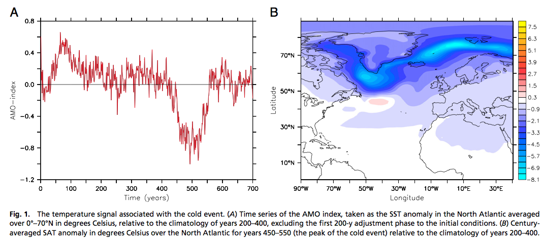
From Drijfhout et al 2013
Figure 1 – Click to expand
In their summary they state:
The lesson learned from this study is that the climate system is capable of generating large, abrupt climate excursions without externally imposed perturbations. Also, because such episodic events occur spontaneously, they may have limited predictability.
Before we look at the “causes” – the climate mechanisms – of this event, let’s briefly look at the climate model.
Their coupled GCM has an atmospheric resolution of just over 1º x 1º with 62 vertical levels, and the ocean has a resolution of 1º in the extra-tropics, increasing to 0.3º near the equator. The ocean has 42 vertical levels, with the top 200m of the ocean represented by 20 equally spaced 10m levels.
The GHGs and aerosols are set at pre-industrial 1860 values and don’t change over the 1,125 year simulation. There are no “flux adjustments” (no need for artificial momentum and energy additions to keep the model stable as with many older models).
See note 1 for a fuller description and the paper in the references for a full description.
The simulated event itself:
After 450 y, an abrupt cooling event occurred, with a clear signal in the Atlantic multidecadal oscillation (AMO). In the instrumental record, the amplitude of the AMO since the 1850s is about 0.4 °C, its SD 0.2 °C. During the event simulated here, the AMO index dropped by 0.8 °C for about a century..
How did this abrupt change take place?
The main mechanism was a change in the Atlantic Meridional Overturning Current (AMOC), also known as the Thermohaline circulation. The AMOC raises a nice example of the sensitivity of climate. The AMOC brings warmer water from the tropics into higher latitudes. A necessary driver of this process is the intensity of deep convection in high latitudes (sinking dense water) which in turn depends on two factors – temperature and salinity. More importantly, more accurately, it depends on the competing differences in anomalies of temperature and salinity
To shut down deep convection, the density of the surface water must decrease. In the temperature range of 7–12 °C, typical for the Labrador Sea, the SST anomaly in degrees Celsius has to be roughly 5 times the sea surface salinity (SSS) anomaly in practical salinity units for density compensation to occur. The SST anomaly was only about twice that of the SSS anomaly; the density anomaly was therefore mostly determined by the salinity anomaly.
In the figure below we see (left) the AMOC time series at two locations with the reduction during the cold century, and (right) the anomaly by depth and latitude for the “cold century” vs the climatology for years 200-400:
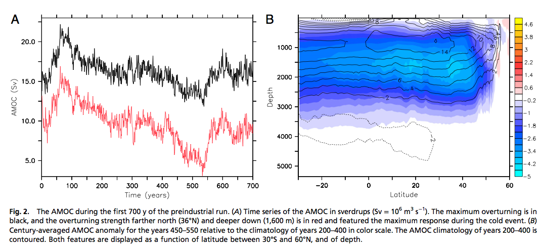
From Drijfhout et al 2013
Figure 2 – Click to expand
What caused the lower salinities? It was more sea ice, melting in the right location. The excess sea ice was caused by positive feedback between atmospheric and ocean conditions “locking in” a particular pattern. The paper has a detailed explanation with graphics of the pressure anomalies which is hard to reduce to anything more succinct, apart from their abstract:
Initial cooling started with a period of enhanced atmospheric blocking over the eastern subpolar gyre.
In response, a southward progression of the sea-ice margin occurred, and the sea-level pressure anomaly was locked to the sea-ice margin through thermal forcing. The cold-core high steered more cold air to the area, reinforcing the sea-ice concentration anomaly east of Greenland.
The sea-ice surplus was carried southward by ocean currents around the tip of Greenland. South of 70°N, sea ice already started melting and the associated freshwater anomaly was carried to the Labrador Sea, shutting off deep convection. There, surface waters were exposed longer to atmospheric cooling and sea surface temperature dropped, causing an even larger thermally forced high above the Labrador Sea.
Conclusion
It is fascinating to see a climate model reproducing an example of abrupt climate change. There are a few contexts to suggest for this result.
1. From the context of timescale we could ask how often these events take place, or what pre-conditions are necessary. The only way to gather meaningful statistics is for large ensemble runs of considerable length – perhaps thousands of “perturbed physics” runs each of 100,000 years length. This is far out of reach for processing power at the moment. I picked some arbitrary numbers – until the statistics start to converge and match what we see from paleoclimatology studies we don’t know if we have covered the “terrain”.
Or perhaps only five runs of 1,000 years are needed to completely solve the problem (I’m kidding).
2. From the context of resolution – as we achieve higher resolution in models we may find new phenomena emerging in climate models that did not appear before. For example, in ice age studies, coarser climate models could not achieve “perennial snow cover” at high latitudes (as a pre-condition for ice age inception), but higher resolution climate models have achieved this first step. (See Ghosts of Climates Past – Part Seven – GCM I & Part Eight – GCM II).
As a comparison on resolution, the 2,000 year El Nino study we saw in Part Six of this series had an atmospheric resolution of 2.5º x 2.0º with 24 levels.
However, we might also find that as the resolution progressively increases (with the inevitable march of processing power) phenomena that appear at one resolution disappear at yet higher resolutions. This is an opinion, but if you ask people who have experience with computational fluid dynamics I expect they will say this would not be surprising.
3. Other models might reach similar or higher resolution and never get this kind of result and demonstrate the flaw in the EC-Earth model that allowed this “Little Ice Age” result to occur. Or the reverse.
As the authors say:
As a result, only coupled climate models that are capable of realistically simulating atmospheric blocking in relation to sea-ice variations feature the enhanced sensitivity to internal fluctuations that may temporarily drive the climate system to a state that is far beyond its standard range of natural variability.
Articles in the Series
Natural Variability and Chaos – One – Introduction
Natural Variability and Chaos – Two – Lorenz 1963
Natural Variability and Chaos – Three – Attribution & Fingerprints
Natural Variability and Chaos – Four – The Thirty Year Myth
Natural Variability and Chaos – Five – Why Should Observations match Models?
Natural Variability and Chaos – Six – El Nino
Natural Variability and Chaos – Seven – Attribution & Fingerprints Or Shadows?
Natural Variability and Chaos – Eight – Abrupt Change
References
Spontaneous abrupt climate change due to an atmospheric blocking–sea-ice–ocean feedback in an unforced climate model simulation, Sybren Drijfhout, Emily Gleeson, Henk A. Dijkstra & Valerie Livina, PNAS (2013) – free paper
EC-Earth V2.2: description and validation of a new seamless earth system prediction model, W. Hazeleger et al, Climate dynamics (2012) – free paper
Notes
Note 1: From the Supporting Information from their paper:
Climate Model and Numerical Simulation. The climate model used in this study is version 2.2 of the EC-Earth earth system model [see references] whose atmospheric component is based on cycle 31r1 of the European Centre for Medium-range Weather Forecasts (ECMWF) Integrated Forecasting System.
The atmospheric component runs at T159 horizontal spectral resolution (roughly 1.125°) and has 62 vertical levels. In the vertical a terrain-following mixed σ/pressure coordinate is used.
The Nucleus for European Modeling of the Ocean (NEMO), version V2, running in a tripolar configuration with a horizontal resolution of nominally 1° and equatorial refinement to 0.3° (2) is used for the ocean component of EC-Earth.
Vertical mixing is achieved by a turbulent kinetic energy scheme. The vertical z coordinate features a partial step implementation, and a bottom boundary scheme mixes dense water down bottom slopes. Tracer advection is accomplished by a positive definite scheme, which does not produce spurious negative values.
The model does not resolve eddies, but eddy-induced tracer advection is parameterized (3). The ocean is divided into 42 vertical levels, spaced by ∼10 m in the upper 200 m, and thereafter increasing with depth. NEMO incorporates the Louvain-la-Neuve sea-ice model LIM2 (4), which uses the same grid as the ocean model. LIM2 treats sea ice as a 2D viscous-plastic continuum that transmits stresses between the ocean and atmosphere. Thermodynamically it consists of a snow and an ice layer.
Heat storage, heat conduction, snow–ice transformation, nonuniform snow and ice distributions, and albedo are accounted for by subgrid-scale parameterizations.
The ocean, ice, land, and atmosphere are coupled through the Ocean, Atmosphere, Sea Ice, Soil 3 coupler (5). No flux adjustments are applied to the model, resulting in a physical consistency between surface fluxes and meridional transports.
The present preindustrial (PI) run was conducted by Met Éireann and comprised 1,125 y. The ocean was initialized from the World Ocean Atlas 2001 climatology (6). The atmosphere used the 40-year ECMWF Re-Analysis of January 1, 1979, as the initial state with permanent PI (1850) greenhouse gas (280 ppm) and aerosol concentrations.


