There are many classes of systems but in the climate blogosphere world two ideas about climate seem to be repeated the most.
In camp A:
We can’t forecast the weather two weeks ahead so what chance have we got of forecasting climate 100 years from now.
And in camp B:
Weather is an initial value problem, whereas climate is a boundary value problem. On the timescale of decades, every planetary object has a mean temperature mainly given by the power of its star according to Stefan-Boltzmann’s law combined with the greenhouse effect. If the sources and sinks of CO2 were chaotic and could quickly release and sequester large fractions of gas perhaps the climate could be chaotic. Weather is chaotic, climate is not.
Of course, like any complex debate, simplified statements don’t really help. So this article kicks off with some introductory basics.
Many inhabitants of the climate blogosphere already know the answer to this subject and with much conviction. A reminder for new readers that on this blog opinions are not so interesting, although occasionally entertaining. So instead, try to explain what evidence is there for your opinion. And, as suggested in About this Blog:
And sometimes others put forward points of view or “facts” that are obviously wrong and easily refuted. Pretend for a moment that they aren’t part of an evil empire of disinformation and think how best to explain the error in an inoffensive way.
Pendulums
The equation for a simple pendulum is “non-linear”, although there is a simplified version of the equation, often used in introductions, which is linear. However, the number of variables involved is only two:
- angle
- speed
and this isn’t enough to create a “chaotic” system.
If we have a double pendulum, one pendulum attached at the bottom of another pendulum, we do get a chaotic system. There are some nice visual simulations around, which St. Google might help interested readers find.
If we have a forced damped pendulum like this one:
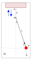
Figure 1 – the blue arrows indicate that the point O is being driven up and down by an external force
-we also get a chaotic system.
What am I talking about? What is linear & non-linear? What is a “chaotic system”?
Digression on Non-Linearity for Non-Technical People
Common experience teaches us about linearity. If I pick up an apple in the supermarket it weighs about 0.15 kg or 150 grams (also known in some countries as “about 5 ounces”). If I take 10 apples the collection weighs 1.5 kg. That’s pretty simple stuff. Most of our real world experience follows this linearity and so we expect it.
On the other hand, if I was near a very cold black surface held at 170K (-103ºC) and measured the radiation emitted it would be 47 W/m². Then we double the temperature of this surface to 340K (67ºC) what would I measure? 94 W/m²? Seems reasonable – double the absolute temperature and get double the radiation.. But it’s not correct.
The right answer is 758 W/m², which is 16x the amount. Surprising, but most actual physics, engineering and chemistry is like this. Double a quantity and you don’t get double the result.
It gets more confusing when we consider the interaction of other variables.
Let’s take riding a bike [updated thanks to Pekka]. Once you get above a certain speed most of the resistance comes from the wind so we will focus on that. Typically the wind resistance increases as the square of the speed. So if you double your speed you get four times the wind resistance. Work done = force x distance moved, so with no head wind power input has to go up as the cube of speed (note 4). This means you have to put in 8x the effort to get 2x the speed.
On Sunday you go for a ride and the wind speed is zero. You get to 25 km/hr (16 miles/hr) by putting a bit of effort in – let’s say you are producing 150W of power (I have no idea what the right amount is). You want your new speedo to register 50 km/hr – so you have to produce 1,200W.
On Monday you go for a ride and the wind speed is 20 km/hr into your face. Probably should have taken the day off.. Now with 150W you get to only 14 km/hr, it takes almost 500W to get to your basic 25 km/hr, and to get to 50 km/hr it takes almost 2,400W. No chance of getting to that speed!
On Tuesday you go for a ride and the wind speed is the same so you go in the opposite direction and take the train home. Now with only 6W you get to go 25 km/hr, to get to 50km/hr you only need to pump out 430W.
In mathematical terms it’s quite simple: F = k(v-w)², Force = (a constant, k) x (road speed – wind speed) squared. Power, P = Fv = kv(v-w)². But notice that the effect of the “other variable”, the wind speed, has really complicated things.
To double your speed on the first day you had to produce eight times the power. To double your speed the second day you had to produce almost five times the power. To double your speed the third day you had to produce just over 70 times the power. All with the same physics.
The real problem with nonlinearity isn’t the problem of keeping track of these kind of numbers. You get used to the fact that real science – real world relationships – has these kind of factors and you come to expect them. And you have an equation that makes calculating them easy. And you have computers to do the work.
No, the real problem with non-linearity (the real world) is that many of these equations link together and solving them is very difficult and often only possible using “numerical methods”.
It is also the reason why something like climate feedback is very difficult to measure. Imagine measuring the change in power required to double speed on the Monday. It’s almost 5x, so you might think the relationship is something like the square of speed. On Tuesday it’s about 70 times, so you would come up with a completely different relationship. In this simple case know that wind speed is a factor, we can measure it, and so we can “factor it out” when we do the calculation. But in a more complicated system, if you don’t know the “confounding variables”, or the relationships, what are you measuring? We will return to this question later.
When you start out doing maths, physics, engineering.. you do “linear equations”. These teach you how to use the tools of the trade. You solve equations. You rearrange relationships using equations and mathematical tricks, and these rearranged equations give you insight into how things work. It’s amazing. But then you move to “nonlinear” equations, aka the real world, which turns out to be mostly insoluble. So nonlinear isn’t something special, it’s normal. Linear is special. You don’t usually get it.
..End of digression
Back to Pendulums
Let’s take a closer look at a forced damped pendulum. Damped, in physics terms, just means there is something opposing the movement. We have friction from the air and so over time the pendulum slows down and stops. That’s pretty simple. And not chaotic. And not interesting.
So we need something to keep it moving. We drive the pivot point at the top up and down and now we have a forced damped pendulum. The equation that results (note 1) has the massive number of three variables – position, speed and now time to keep track of the driving up and down of the pivot point. Three variables seems to be the minimum to create a chaotic system (note 2).
As we increase the ratio of the forcing amplitude to the length of the pendulum (β in note 1) we can move through three distinct types of response:
- simple response
- a “chaotic start” followed by a deterministic oscillation
- a chaotic system
This is typical of chaotic systems – certain parameter values or combinations of parameters can move the system between quite different states.
Here is a plot (note 3) of position vs time for the chaotic system, β=0.7, with two initial conditions, only different from each other by 0.1%:

Forced damped harmonic pendulum, b=0.7: Start angular speed 0.1; 0.1001
Figure 1
It’s a little misleading to view the angle like this because it is in radians and so needs to be mapped between 0-2π (but then we get a discontinuity on a graph that doesn’t match the real world). We can map the graph onto a cylinder plot but it’s a mess of reds and blues.
Another way of looking at the data is via the statistics – so here is a histogram of the position (θ), mapped to 0-2π, and angular speed (dθ/dt) for the two starting conditions over the first 10,000 seconds:
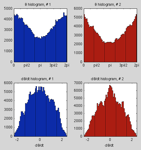
Histograms for 10,000 seconds
Figure 2
We can see they are similar but not identical (note the different scales on the y-axis).
That might be due to the shortness of the run, so here are the results over 100,000 seconds:
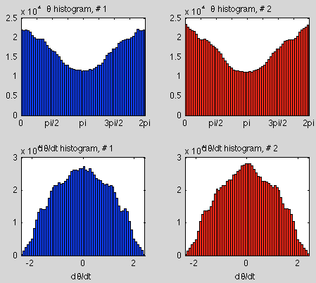
Histogram for 100,000 seconds
Figure 3
As we increase the timespan of the simulation the statistics of two slightly different initial conditions become more alike.
So if we want to know the state of a chaotic system at some point in the future, very small changes in the initial conditions will amplify over time, making the result unknowable – or no different from picking the state from a random time in the future. But if we look at the statistics of the results we might find that they are very predictable. This is typical of many (but not all) chaotic systems.
Orbits of the Planets
The orbits of the planets in the solar system are chaotic. In fact, even 3-body systems moving under gravitational attraction have chaotic behavior. So how did we land a man on the moon? This raises the interesting questions of timescales and amount of variation. Planetary movement – for our purposes – is extremely predictable over a few million years. But over 10s of millions of years we might have trouble predicting exactly the shape of the earth’s orbit – eccentricity, time of closest approach to the sun, obliquity.
However, it seems that even over a much longer time period the planets will still continue in their orbits – they won’t crash into the sun or escape the solar system. So here we see another important aspect of some chaotic systems – the “chaotic region” can be quite restricted. So chaos doesn’t mean unbounded.
According to Cencini, Cecconi & Vulpiani (2010):
Therefore, in principle, the Solar system can be chaotic, but not necessarily this implies events such as collisions or escaping planets..
However, there is evidence that the Solar system is “astronomically” stable, in the sense that the 8 largest planets seem to remain bound to the Sun in low eccentricity and low inclination orbits for time of the order of a billion years. In this respect, chaos mostly manifest in the irregular behavior of the eccentricity and inclination of the less massive planets, Mercury and Mars. Such variations are not large enough to provoke catastrophic events before extremely large time. For instance, recent numerical investigations show that for catastrophic events, such as “collisions” between Mercury and Venus or Mercury failure into the Sun, we should wait at least a billion years.
And bad luck, Pluto.
Deterministic, non-Chaotic, Systems with Uncertainty
Just to round out the picture a little, even if a system is not chaotic and is deterministic we might lack sufficient knowledge to be able to make useful predictions. If you take a look at figure 3 in Ensemble Forecasting you can see that with some uncertainty of the initial velocity and a key parameter the resulting velocity of an extremely simple system has quite a large uncertainty associated with it.
This case is quantitively different of course. By obtaining more accurate values of the starting conditions and the key parameters we can reduce our uncertainty. Small disturbances don’t grow over time to the point where our calculation of a future condition might as well just be selected from a randomly time in the future.
Transitive, Intransitive and “Almost Intransitive” Systems
Many chaotic systems have deterministic statistics. So we don’t know the future state beyond a certain time. But we do know that a particular position, or other “state” of the system, will be between a given range for x% of the time, taken over a “long enough” timescale. These are transitive systems.
Other chaotic systems can be intransitive. That is, for a very slight change in initial conditions we can have a different set of long term statistics. So the system has no “statistical” predictability. Lorenz 1968 gives a good example.
Lorenz introduces the concept of almost intransitive systems. This is where, strictly speaking, the statistics over infinite time are independent of the initial conditions, but the statistics over “long time periods” are dependent on the initial conditions. And so he also looks at the interesting case (Lorenz 1990) of moving between states of the system (seasons), where we can think of the precise starting conditions each time we move into a new season moving us into a different set of long term statistics. I find it hard to explain this clearly in one paragraph, but Lorenz’s papers are very readable.
Conclusion?
This is just a brief look at some of the basic ideas.
Articles in the Series
Natural Variability and Chaos – One – Introduction
Natural Variability and Chaos – Two – Lorenz 1963
Natural Variability and Chaos – Three – Attribution & Fingerprints
Natural Variability and Chaos – Four – The Thirty Year Myth
Natural Variability and Chaos – Five – Why Should Observations match Models?
Natural Variability and Chaos – Six – El Nino
Natural Variability and Chaos – Seven – Attribution & Fingerprints Or Shadows?
Natural Variability and Chaos – Eight – Abrupt Change
References
Chaos: From Simple Models to Complex Systems, Cencini, Cecconi & Vulpiani, Series on Advances in Statistical Mechanics – Vol. 17 (2010)
Climatic Determinism, Edward Lorenz (1968) – free paper
Can chaos and intransivity lead to interannual variation, Edward Lorenz, Tellus (1990) – free paper
Notes
Note 1 – The equation is easiest to “manage” after the original parameters are transformed so that tω->t. That is, the period of external driving, T0=2π under the transformed time base.
Then:

where θ = angle, γ’ = γ/ω, α = g/Lω², β =h0/L;
these parameters based on γ = viscous drag coefficient, ω = angular speed of driving, g = acceleration due to gravity = 9.8m/s², L = length of pendulum, h0=amplitude of driving of pivot point
Note 2 – This is true for continuous systems. Discrete systems can be chaotic with less parameters
Note 3 – The results were calculated numerically using Matlab’s ODE (ordinary differential equation) solver, ode45.
Note 4 – Force = k(v-w)2 where k is a constant, v=velocity, w=wind speed. Work done = Force x distance moved so Power, P = Force x velocity.
Therefore:
P = kv(v-w)2
If we know k, v & w we can find P. If we have P, k & w and want to find v it is a cubic equation that needs solving.


Small supplement
“We have friction from the air and so over time the pendulum slows down and stops.”
By the friction decreases, the amplitude, but the period is shorter:
https://commons.wikimedia.org/wiki/File:Pendulum_period.svg
I should fix up my sloppy definition about the number of variables in the pendulum equations. Time is a variable of course in the equation for the simple pendulum.
For a system of ordinary differential equations:
dx1/dt = f1(x1, x2,.. xn)
dx2/dt = f2(x1, x2,.. xn)
..
dxn/dt = fn(x1, x2,.. xn)
there are n dependent variables so the system dimension, d = n.
If we add time as a dependent variable in the ODEs (e.g., dx1/dt = f1(x1, x2,.. xn, t) then the system dimension, d = n+1.
When the system dimension, d ≥ 3 and the equations are non-linear then the system can be chaotic.
A linear system will be of the form of:
dx1/dt = a1.x1 + b1.x2 +c1.x3 and so on (where a1, b1, c1 etc are constants). These systems can’t be chaotic.
A nonlinear system will be something like:
dx1/dt = a1.x22 – x1.x3
SoD,
You didn’t think carefully about your biking example.
The power you need in cycling is velocity x resistance. Thus it grows in third power of velocity in calm weather. 50 km/h takes 1200 W. in your case of headwind you get to the speed of 13.7 km/h with 150 W, and 25 km/h with 486 W.
Pekka,
I believe you are correct.
Which might explain why in my head as I started writing I was firmly of the opinion that the ratio was P = kv3, but when I checked a cycling article, forgetting physics basics, I found the wind resistance “force” was v2 and just assumed my memory had been at fault..
I will update the article. The more non-linearity the better as far as the takeaways are concerned.
It depends a bit on what you mean by effort. If two riders complete a 30 km training run in still air on level ground and A rides twice as fast as B then I think one would say that A put in 4 times as much effort into the run as B. In this case one would be using effort to mean work done. If they both rode for the same amount of time, rather than the same distance, then the ratio would be 8.
Pekka is entitled to regard effort as being equivalent to power, but I think that equating it with work is at least equally valid.
You also left off cumulative error from rounding because you can’t calculate to infinite precision. That can cause problems even in linear systems over sufficient time.
It appears much of the temperature anomaly for the 97/98 El Nino is due to albedo. And it appears that the albedo difference is due to pattern of circulation ( difference in location and amount of clouds from storm tracks ).
El Nino events are brief in the context of climate, but frequencies of El Ninos, ( a couple more per century ) are enough to change temperature trends. And other more poorly understood fluctuations ( PDO, AMO, etc. ) evidently also exert an influence.
I would think that the forcing from CO2 is relatively predictable, but that climate as a whole would be still subject to the non-linearities as weather, just those of longer time scales.
I think I see where this is heading, but it misses some critical points. First, we know the basic source of forces (exactly for the main ones) on pendulums and planets, it is just the coupled non-linearity and lack of perfect initial condition data, and small stray external effects that produce the long term real vs. calculation errors in such chaotic systems. As pointed out, these are simple enough problems and stray external forces small enough so that either long term to very long times or statistical average values can be satisfactorily determined in some cases.
Climate has much more complexity and lack of understanding that would limit long term prediction capability. The first and foremost is that not all of the important physical details and thus maths are even adequately known. These include the full effects of clouds, aerosols, long period ocean currents, solar spectral variation and feedback effects on the system. In addition, boundary conditions can change somewhat over time (cutting forests, building cities, dams, etc.) and computation grids cannot be made to nearly adequate resolution. For a very complex combination of numerous non-linear drivers and interactions, and even variable boundary conditions, this makes what appears to be an intractable chaotic system. Short term weather cannot be determined more that a few days at most and long term (centuries long) climate calculations have no real chance. Only intermediate lengths calculations (a few decades) even have a chance, but only if the physical processes and grid resolution could be greatly improved (far beyond what I think likely).
The problem is that scary claims were made based on this unrealistic claim of knowing the process, and that has caused fear and spending of large sums of money that have show no value. Loans to third world countries to build coal power plants were stopped, negatively impacting the people. The effort to understand the CO2 increase and temporary temperature increase were needed, but badly misused, and efforts to see if natural variation was important here were often not funded, since the emphasis was only on CO2. Now claims are being made that the pause is natural variation (who knew), and is likely only temporary?
Leonard,
No, we don’t. For the pendulum, local g varies daily because of the lunar and solar tidal effect. Lunar orbital eccentricity cannot even be predicted accurately. Air friction will vary with atmospheric density, which is a function of temperature, humidity and barometric pressure. None of these are known exactly. And that’s ignoring the frictional contribution from the pivot points. We only know exactly a mathematical model of a coupled pendulum, not a real pendulum. There are similar problems with the real solar system.
DeWitt
I may not have stated clearly enough what I was attempting to say. When I said exactly. I was referring to the nature of the physics of the gravity effects. That is why I also added there were stray external effects (air friction, pivot friction, air density, weak gravitational perturbations from distant bodies, etc.), and lack of EXACT initial conditions (value of gravity, location). For climate, we do not even have all of the physics.
SOD: If I understand Figure 1 and the comment underneath, your forced pendulum has made 40+ full rotations (250 radians) in the positive direction. Does this system behave like a random walk, with the “distance” from the starting position growing with time with the square root of time? If so, it’s not a great model for the chaotic behavior of climate on a planet not likely to experience a runaway greenhouse effect. That is my objection to Doug Kennan’s statistical models that fit the history of 20th century warming better than the linear AR1 models used by the IPCC to characterize century-wide warming trends. I the future I hope you exemplify chaotic behavior with a model that doesn’t show random walk behavior.
If you choose a pendulum with a smaller driving force, you would probably get oscillations without full rotations. You could increase the driving force and see the average kinetic energy (“temperature”) increase. But I suspect these oscillations wouldn’t show chaotic behavior.
The earth obviously receives a large cyclic driving force from seasonal changes in radiation, but all not all “pendulums” (ENSO, MJO, AMO etc.) oscillate with a natural frequency of about 1 year. Apparently ENSO is often triggered at about the same time in the annual cycle, but only managers to switch modes every few years. It doesn’t seem as if there are cyclic driving forces with an appropriate frequency to drive the AMO or a LIA with a natural frequency of several decades or several centuries.
Frank,
It doesn’t have random walk characteristics.
It’s not a good analogy for the climate system at all. It’s just the one of the simplest chaotic systems to look at.
I’m not attempting to draw any conclusions at all from the forced damped pendulum, just to illustrate chaos in time but repeatability in statistics in a very simple chaotic system.
I am looking forward to the next Ghosts of Climate Past installment. With a decadel or bi-decadel mean temperature, I’ll ask what about a 1000 years mean? I am a chaos theory person but without a lot of knowledge on the subject. Pushing the time frame to 100,000 years, here’s from your #19 Ghosts of Climate Past,
“Increased dynamical activity of the ice sheet would lead to net thinning of the ice sheet interior and the transport of large amounts of ice into regions of intense ablation both south of the ice sheet and at the marine margins (via calving). This has the potential to provide a strong positive feedback on deglaciation.”
I thank you for pointing this out. It’s part of what strengthened my opinion about chaos. I see the above as, you can only stack ice so high, then basal sliding takes over. It’s an avalanche that may initiate change. It’s an elegant answer with sea levels dropping with water moving to land in the form of ice, then it fixes itself with a collapse. I think my point is, what was the mean decadel temperature when the above collapse was under way when were leaving the glacial phase? It this is better left to next the installment, I understand.
SOD summarized the Camp B position as “…If the sources and sinks of CO2 were chaotic and could quickly release and sequester large fractions of gas perhaps the climate could be chaotic. Weather is chaotic, climate is not.”
A more sensible alternative might be: The ocean is provides a huge reservoir of stratified water that is much colder than the average surface temperature. Climate almost certainly is chaotic because heat exchange between the mixed layer and the deeper ocean is mediated of ocean currents and the equations that describe fluid flow generally have chaotic solutions. ENSO, for example, is driven by a chaotic exchange of heat between the deeper portions of the Western Pacific Warm Pool and the surface of the colder Eastern Pacific. Chaotic behavior almost certainly exists; but the amplitude of the temperature change associated with such chaos is unknown.
Frankon July 26, 2014 at 11:35 pm
“… but the amplitude of the temperature change associated with such chaos is unknown.”
However, the average value is known. And the average value is not chaotic. The deviations from the average value are very often a normal distribution, because the events (deviations) have many independent causes – central limit theorem of statistics.
Ebel: How long can temperature deviate from average values? Was the LIA, which lasted 500 years, caused by a reduction in forcing or unforced variability (or some of both). There certainly were some forcing changes (volcanos, the Maunder and Dalton solar minimums), but it isn’t clear to me that they account for all of the cold (unless climate sensitivity is very high). If one can’t be sure unforced variability didn’t contribute to the LIA, then the warming in the last few decades of the 20th century doesn’t appear to be unusual.
[…] « Natural Variability and Chaos – One – Introduction […]
“All laws of nature are local.” So we might say climate is an aggregation of all weather, and the way to get to climate is a bottom up approach. “At what scales does the climate start?” Applying different time and space definitions can be arbitrary and cause one to miss what is happening. If weather is chaotic, it follows that climate is.
The quotes are from Tomas Milanovic at:
[…] Part One and Part Two we had a look at chaotic systems and what that might mean for weather and climate. I […]
[…] learnt from simple chaotic systems, like the Lorenz 1963 model. There is discussion of this in Part One and Part Two of this series. As some commenters have pointed out that doesn’t mean the […]
[…] introduction to attribution studies, chaos and natural variability here in a eight part series. Natural Variability and Chaos – One – Introduction | The Science of Doom Yu Kosaka & Shang-Ping Xie, as published in Nature (Nature Publishing Group : science […]
[…] people unfamiliar with chaotic systems, it is worth reading Natural Variability and Chaos – One – Introduction and Natural Variability and Chaos – Two – Lorenz 1963. The Lorenz system of three equations […]