In Part Seven – Resolution & Convection we looked at some examples of how model resolution and domain size had big effects on modeled convection.
One commenter highlighted some presentations on issues in GCMs. As there were already a lot of comments on that article the relevant points appear a long way down. The issue deserves at least a short article of its own.
The presentations, by Paul Williams, Department of Meteorology, University of Reading, UK – all freely available:
The impacts of stochastic noise on climate models
The importance of numerical time-stepping errors
The leapfrog is dead. Long live the leapfrog!
Various papers are highlighted in these presentations (often without a full reference).
Time-Step Dependence
One of the papers cited: Time Step Sensitivity of Nonlinear Atmospheric Models: Numerical Convergence, Truncation Error Growth, and Ensemble Design, Teixeira, Reynolds & Judd 2007 comments first on the Lorenz equations (see Natural Variability and Chaos – Two – Lorenz 1963):
Figure 3a shows the evolution of X for r =19 for three different time steps (10-2, 10-3, and 10-4 LTU).
In this regime the solutions exhibit what is often referred to as transient chaotic behavior (Strogatz 1994), but after some time all solutions converge to a stable fixed point.
Depending on the time step used to integrate the equations, the values for the fixed points can be different, which means that the climate of the model is sensitive to the time step.
In this particular case, the solution obtained with 0.01 LTU converges to a positive fixed point while the other two solutions converge to a negative value.
To conclude the analysis of the sensitivity to parameter r, Fig. 3b shows the time evolution (with r =21.3) of X for three different time steps. For time steps 0.01 LTU and 0.0001 LTU the solution ceases to have a chaotic behavior and starts converging to a stable fixed point.
However, for 0.001 LTU the solution stays chaotic, which shows that different time steps may not only lead to uncertainty in the predictions after some time, but may also lead to fundamentally different regimes of the solution.
These results suggest that time steps may have an important impact in the statistics of climate models in the sense that something relatively similar may happen to more complex and realistic models of the climate system for time steps and parameter values that are currently considered to be reasonable.
[Emphasis added]
For people unfamiliar with chaotic systems, it is worth reading Natural Variability and Chaos – One – Introduction and Natural Variability and Chaos – Two – Lorenz 1963. The Lorenz system of three equations creates a very simple system of convection where we humans have the advantage of god-like powers. Although, as this paper shows, it seems that even with our god-like powers, under certain circumstances, we aren’t able to confirm
- the average value of the “climate”, or even
- if the climate is a deterministic or chaotic system
The results depend on the time step we have used to solve the set of equations.
Then the paper then goes on to consider a couple of models, including a weather forecasting model. In their summary:
In the weather and climate prediction community, when thinking in terms of model predictability, there is a tendency to associate model error with the physical parameterizations.
In this paper, it is shown that time truncation error in nonlinear models behaves in a more complex way than in linear or mildly nonlinear models and that it can be a substantial part of the total forecast error.
The fact that it is relatively simple to test the sensitivity of a model to the time step, allowed us to study the implications of time step sensitivity in terms of numerical convergence and error growth in some depth. The simple analytic model proposed in this paper illustrates how the evolution of truncation error in nonlinear models can be understood as a combination of the typical linear truncation error and of the initial condition error associated with the error committed in the first time step integration (proportional to some power of the time step).
A relevant question is how much of this simple study of time step truncation error could help in understanding the behavior of more complex forms of model error associated with the parameterizations in weather and climate prediction models, and its interplay with initial condition error.
Another reference from the presentations is Dependence of aqua-planet simulations on time step, Willamson & Olsen 2003.
What is an aquaplanet simulation?
In an aqua-planet the earth is covered with water and has no mountains. The sea surface temperature (SST) is specied, usually with rather simple geometries such as zonal symmetry. The ‘correct’ solutions of aqua-planet tests are not known.
However, it is thought that aqua-planet studies might help us gain insight into model differences, understand physical processes in individual models, understand the impact of changing parametrizations and dynamical cores, and understand the interaction between dynamical cores and parametrization packages. There is a rich history of aqua-planet experiments, from which results relevant to this paper are discussed below.
They found that running different “mechanisms” for the same parameterizations produced quite different precipitation results. In investigating further it appeared that the time step was the key change.
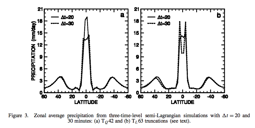
Figure 1 – Click to enlarge
Their conclusion:
When running the Neale and Hoskins (2000a) standard aqua-planet test suite with two versions of the CCM3, which differed in the formulation of the dynamical cores, we found a strong sensitivity in the morphology of the time averaged, zonal averaged precipitation.
The two dynamical cores were candidates for the successor model to CCM3; one was Eulerian and the other semi-Lagrangian.
They were each configured as proposed for climate simulation application, and believed to be of comparable accuracy.
The major difference was computational efficiency. In general, simulations with the Eulerian core formed a narrow single precipitation peak centred on the equator, while those with the semi-Lagrangian core produced more precipitation farther from the equator accompanied by a double peak straddling the equator with a minimum centred on the equator..
..We do not know which simulation is ‘correct’. Although a single peak forms with smaller time steps, the simulations do not converge with the smallest time step considered here. The maximum precipitation rate at the equator continues to increase..
..The significance of the time truncation error of parametrizations deserves further consideration in AGCMs forced by real-world conditions.
Stochastic Noise
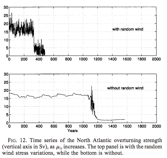
From Global Thermohaline Circulation. Part I: Sensitivity to Atmospheric Moisture Transport, Xiaoli Wang et al 1999, the strength of the North Atlantic overturning current (the thermohaline circulation) changed significantly with noise:
From Wang et al 1999
Figure 2
The idea behind the experiment is that increasing freshwater fluxes at high latitudes from melting ice (in a warmer world) appear to impact the strength of the Atlantic “conveyor” which brings warm water from nearer the equator to northern Europe (there is a long history of consideration of this question). How sensitive is this to random effects?
In these experiments we also include random variations in the zonal wind stress field north of 46ºN. The variations are uniform in space and have a Gaussian distribution, with zero mean and standard deviation of 1 dyn/cm² , based on European Centre for MediumRange Weather Forecasts (ECMWF) analyses (D. Stammer 1996, personal communication).
Our motivation in applying these random variations in wind stress is illustrated by two experiments, one with random wind variations, the other without, in which μN increases according to the above prescription. Figure 12 shows the time series of the North Atlantic overturning strength in these two experiments. The random wind variations give rise to interannual variations in the strength of the overturning, which are comparable in magnitude to those found in experiments with coupled GCMs (e.g., Manabe and Stouffer 1994), whereas interannual variations are almost absent without them. The variations also accelerate the collapse of the overturning, therefore speeding up the response time of the model to the freshwater flux perturbation (see Fig. 12). The reason for the acceleration of the collapse is that the variations make it harder for the convection to sustain itself.
The convection tends to maintain itself, because of a positive feedback with the overturning circulation (Lenderink and Haarsma 1994). Once the convection is triggered, it creates favorable conditions for further convection there. This positive feedback is so powerful that in the case without random variations the convection does not shut off until the freshening is virtually doubled at the convection site (around year 1000). When the random variations are present, they generate perturbations in the Ekman currents, which are propagated downward to the deep layers, and cause variations in the overturning strength. This weakens the positive feedback.
In general, the random wind stress variations lead to a more realistic variability in the convection sites, and in the strength of the overturning circulation.
We note that, even though the transitions are speeded up by the technique, the character of the model behavior is not fundamentally altered by including the random wind variations.
The presentation on stochastic noise also highlighted a coarse resolution GCM that didn’t show El-Nino features – but after the introduction of random noise it did.
I couldn’t track down the reference – Joshi, Williams & Smith 2010 – and emailed Paul Williams who replied very quickly, and helpfully – the paper is still “in preparation” so that means it probably won’t ever be finished, but instead Paul pointed me to two related papers that had been published: Improved Climate Simulations through a Stochastic Parameterization of Ocean Eddies – Paul D Williams et al, AMS (2016) and Climatic impacts of stochastic fluctuations in air–sea fluxes, Paul D Williams et al, GRL (2012).
From the 2012 paper:
In this study, stochastic fluctuations have been applied to the air–sea buoyancy fluxes in a comprehensive climate model. Unlike related previous work, which has employed an ocean general circulation model coupled only to a simple empirical model of atmospheric dynamics, the present work has employed a full coupled atmosphere–ocean general circulation model. This advance allows the feedbacks in the coupled system to be captured as comprehensively as is permitted by contemporary high-performance computing, and it allows the impacts on the atmospheric circulation to be studied.
The stochastic fluctuations were introduced as a crude attempt to capture the variability of rapid, sub-grid structures otherwise missing from the model. Experiments have been performed to test the response of the climate system to the stochastic noise.
In two experiments, the net fresh water flux and the net heat flux were perturbed separately. Significant changes were detected in the century-mean oceanic mixed-layer depth, sea-surface temperature, atmospheric Hadley circulation, and net upward water flux at the sea surface. Significant changes were also detected in the ENSO variability. The century-mean changes are summarized schematically in Figure 4. The above findings constitute evidence that noise-induced drift and noise-enhanced variability, which are familiar concepts from simple models, continue to apply in comprehensive climate models with millions of degrees of freedom..
The graph below shows the control experiment (top) followed by the difference between two experiments and the control (note change in vertical axis scale for the two anomaly experiments) where two different methods of adding random noise were included:
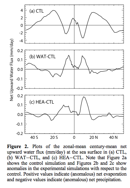
From Williams et al 2012
Figure 3
A key element of the paper is that adding random noise changes the mean values.
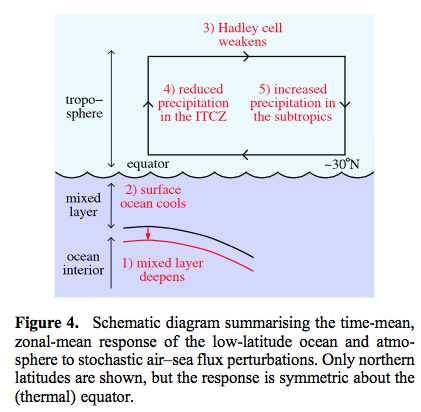
From Williams et al 2012
Figure 4
From the 2016 paper:
Faster computers are constantly permitting the development of climate models of greater complexity and higher resolution. Therefore, it might be argued that the need for parameterization is being gradually reduced over time.
However, it is difficult to envisage any model ever being capable of explicitly simulating all of the climatically important components on all of the relevant time scales. Furthermore, it is known that the impact of the subgrid processes cannot necessarily be made vanishingly small simply by increasing the grid resolution, because information from arbitrarily small scales within the inertial subrange (down to the viscous dissipation scale) will always be able to contaminate the resolved scales in finite time.
This feature of the subgrid dynamics perhaps explains why certain systematic errors are common to many different models and why numerical simulations are apparently not asymptoting as the resolution increases. Indeed, the Intergovernmental Panel on Climate Change (IPCC) has noted that the ultimate source of most large-scale errors is that ‘‘many important small- scale processes cannot be represented explicitly in models’’.
And they continue with an excellent explanation:
The major problem with conventional, deterministic parameterization schemes is their assumption that the impact of the subgrid scales on the resolved scales is uniquely determined by the resolved scales. This assumption can be made to sound plausible by invoking an analogy with the law of large numbers in statistical mechanics.
According to this analogy, the subgrid processes are essentially random and of sufficiently large number per grid box that their integrated effect on the resolved scales is predictable. In reality, however, the assumption is violated because the most energetic subgrid processes are only just below the grid scale, placing them far from the limit in which the law of large numbers applies. The implication is that the parameter values that would make deterministic parameterization schemes exactly correct are not simply uncertain; they are in fact indeterminate.
Later:
The question of whether stochastic closure schemes outperform their deterministic counterparts was listed by Williams et al. (2013) as a key outstanding challenge in the field of mathematics applied to the climate system.
Adding noise with a mean zero doesn’t create a mean zero effect?
The changes to the mean climatological state that were identified in section 3 are a manifestation of what, in the field of stochastic dynamical systems, is called noise-induced drift or noise-induced rectification. This effect arises from interactions between the noise and nonlinearities in the model equations. It permits zero- mean noise to have non-zero-mean effects, as seen in our stochastic simulations.
The paper itself aims..
..to investigate whether climate simulations can be improved by implementing a simple stochastic parameterization of ocean eddies in a coupled atmosphere–ocean general circulation model.
The idea is whether adding noise can improve model results more effectively than increasing model resolution:
We conclude that stochastic ocean perturbations can yield reductions in climate model error that are comparable to those obtained by refining the resolution, but without the increased computational cost.
In this latter respect, our findings are consistent with those of Berner et al. (2012), who studied the model error in an atmospheric general circulation model. They reported that, although the impact of adding stochastic noise is not universally beneficial in terms of model bias reduction, it is nevertheless beneficial across a range of variables and diagnostics. They also reported that, in terms of improving the magnitudes and spatial patterns of model biases, the impact of adding stochastic noise can be similar to the impact of increasing the resolution. Our results are consistent with these findings. We conclude that oceanic stochastic parameterizations join atmospheric stochastic parameterizations in having the potential to significantly improve climate simulations.
And for people who’ve been educated on the basics of fluids on a rotating planet via experiments on the rotating annulus (a 2d model – along with equations – providing great insights into our 3d planet), Testing the limits of quasi-geostrophic theory: application to observed laboratory flows outside the quasi-geostrophic regime, Paul D Williams et al 2010 might be interesting.
Conclusion
Some systems have a lot of non-linearity. This is true of climate and generally of turbulent flows.
In a textbook that I read some time ago on (I think) chaos, the author made the great comment that usually you start out being taught “linear models” and much later come into contact with “non-linear models”. He proposed that a better terminology would be “real world systems” (non-linear) while “simplistic non-real-world teaching models” were the alternative (linear models). I’m paraphrasing.
The point is that most real world systems are non-linear. And many (not all) non-linear systems have difficult properties. The easy stuff you learn – linear systems, aka “simplistic non-real-world teaching models” – isn’t actually relevant to most real world problems, it’s just a stepping stone in giving you the tools to solve the hard problems.
Solving these difficult systems requires numerical methods (there is mostly no analytical solution) and once you start playing around with time-steps, parameter values and model resolution you find that the results can be significantly – and sometimes dramatically – affected by the arbitrary choices. With relatively simple systems (like the Lorenz three-equation convection system) and massive computing power you can begin to find the dependencies. But there isn’t a clear path to see where the dependencies lie (of course, many people have done great work in systematizing (simple) chaotic systems to provide some insights).
GCMs provide insights into climate that we can’t get otherwise.
One way to think about GCMs is that once they mostly agree on the direction of an effect that provides “high confidence”, and anyone who doesn’t agree with that confidence is at best a cantankerous individual and at worst has a hidden agenda.
Another way to think about GCMs is that climate models are mostly at the mercy of unverified parameterizations and numerical methods and anyone who does accept their conclusions is naive and doesn’t appreciate the realities of non-linear systems.
Life is complex and either of these propositions could be true, along with anything inbetween.
More about Turbulence: Turbulence, Closure and Parameterization
References
Time Step Sensitivity of Nonlinear Atmospheric Models: Numerical Convergence, Truncation Error Growth, and Ensemble Design, Teixeira, Reynolds & Judd, Journal of the Atmospheric Sciences (2007) – free paper
Dependence of aqua-planet simulations on time step, Willamson & Olsen, Q. J. R. Meteorol. Soc. (2003) – free paper
Global Thermohaline Circulation. Part I: Sensitivity to Atmospheric Moisture Transport, Xiaoli Wang, Peter H Stone, and Jochem Marotzke, American Meteorological Society (1999) – free paper
Improved Climate Simulations through a Stochastic Parameterization of Ocean Eddies – Paul D Williams et al, AMS (2016) – free paper
Climatic impacts of stochastic fluctuations in air–sea fluxes, Paul D Williams et al, GRL (2012) – free paper
Testing the limits of quasi-geostrophic theory: application to observed laboratory flows outside the quasi-geostrophic regime, Paul Williams, Peter Read & Thomas Haine, J. Fluid Mech. (2010) – free paper


I’m glad you have communicated with him directly.
Dithering, the purposeful addition of noise, is used in digital audio and video processing to reduce some artefacts.
https://en.wikipedia.org/wiki/Dither
So adding noise to improve results isn’t exactly a new idea. It traces back to at least WWII:
I found it difficult to grasp as it is heavy theoretical stuff. Found some concretization in a paper of Sungduk Yu and Michael S. Pritchard about CAM models. The effect of large-scale model time step and multiscale coupling frequency on cloud climatology, vertical structure, and rainfall extremes in a superparameterized GCM (2015)
http://onlinelibrary.wiley.com/doi/10.1002/2015MS000493/pdf
Very nice writeup SOD. I also looked back at the turbulence post. Also well done.
I personally think we really need some new theoretical work on attractors, shadowing methods etc. I believe we could run numerical simulations with current methods for a long time without ever learning anything fundamental. I would point out that there are a few CFD codes out there that use Newton’s method. Those codes have actually helped us uncover fundamental facts such as the prominance of multiple solutions in CFD. There has really been virtually no progress on finite volume methods in 30 years. Like so many lines of scientific research, there are tens of thousands of papers and virtually all are not forgotten because they are microscopic “improvements” demonstrated with cherry picking. That’s how science dies, not with a bang but with a wimper.
Re the conclusion section: you have left out the key role observations play in evaluating model predictions. In climate science observations plus modeling is generally needed for “high” confidence. Where models do not agree with observation there is generally “low or no” confidence.
Stronger turbulence causes a stir – Paul Williams and Luke Storer
JCH,
Thanks for the blog link – this looks like an excellent blog (new to me).
A recent article that looks very relevant to recent articles in this series is Chaotic Convection
Yes, I read that one when I found the Williiams blog. The internet is so full of stuff it just never ends. Anyway, I doubt that Williams would agree with a lot of things being said here.
Excellent post!
I wonder if time step differences also account for the differences between the various reanalyses.
I recently came across this view of radiosondes, reanalyses and GCMs.
Interesting reference. Thank you TE.
Is there a good table of GCM model spatial and temporal resolutions used over time?
SOD concluded:
“One way to think about GCMs is that once they mostly agree on the direction of an effect that provides “high confidence”, and anyone who doesn’t agree with that confidence is at best a cantankerous individual and at worst has a hidden agenda.
Another way to think about GCMs is that climate models are mostly at the mercy of unverified parameterizations and numerical methods and anyone who does accept their conclusions is naive and doesn’t appreciate the realities of non-linear systems.
Life is complex and either of these propositions could be true, along with anything inbetween.”
Let’s compare weather prediction models to AOGCMs. To some extent, weather prediction models have the same weaknesses: “parameterization and numerical methods”. However, SOD added one key word: “UNVERIFIED parameterization and numerical methods”. In the case of weather prediction, the parameters and methods are verified for a time frame of a week by observations – until the point where initialization uncertainty and chaos combine to make day-to-day changes unpredictable. Perhaps parameter uncertainty and “numerical” uncertainty (time step size) also contribute to this failure. However, if we ran weather prediction models for a whole year (and the model didn’t drift upward or downward over the years), the unforced variations we see from day-to-day would presumably appear to be fairly trivial compared with the warming the model should be able to forecast from winter to summer. That is because unforced variability is much smaller that the forced variability from changing solar irradiation.
For climate models to be useful, they need to be able to handle forced variability driven by rising GHGs. Experience tells us that the unforced variability/chaos expected from ENSO and related phenomena is likely to be relatively unimportant compared with forced change is climate sensitivity is high. This would even be true if the LIA and MWP were unforced variability. The inability of AOGCMs to properly deal with chaos/unforced variability may not be critical.
One way to test this is to see how well AOGCMs predict the feedbacks associated with seasonal warming, which is comparable to global warming. Suppose climate models were someday able to gets average seasonal changes in climate and feedbacks correct (which they don’t do today). Given what we know about the modest chaotic fluctuations in climate throughout the Holocene, why wouldn’t we accept larger projections of forced warming?
Well Frank, I agree with your seasonal feedbacks being a necessary condition for accepting GCM predictions. It is NOT a sufficient condition however.
What this post is about is how in the very long term, inaccuracies can build up and lead to different climates. This should be obvious to any climate scientist who has even a passing training in CFD for example.
I stated above what we really need to be able to trust such simulations. It is not a matter of just running more simulations, increasing “resolution”, or better sub grid models of ill-posed processes.
One thing that can be confidently asserted is that many climate scientists are grossly overconfident in GCM results especially on issues like clouds and precipitation and convection. Isaac Held as much as admitted that he had fallen victim to this bias himself.
Isaac Held as much as admitted that he had fallen victim to this bias himself.
Can you provide aline to what you are talking about? Held has not blogged in over a year.
Frank referenced it earlier.
https://www.gfdl.noaa.gov/blog_held/60-the-quality-of-the-large-scale-flow-simulated-in-gcms/
“You can err on the side of inappropriately dismissing model results; this is often the result of being unaware of what these models are and of what they do simulate with considerable skill and of our understanding of where the weak points are. But you can also err on the side of uncritical acceptance of model results; this can result from being seduced by the beauty of the simulations and possibly by a prior research path that was built on utilizing model strengths and avoiding their weaknesses (speaking of myself here).”
Basically, Rossby waves are well simulated, but lots of other stuff is not.
He stopped blogging over a year ago. At about the same time skeptic blogs were using his quotes. I think he expressed some disapproval of that.
Anyway, you have jumped to a conclusion that he has not made, and I sincerely doubt he would agree with.
dpy6629: Thanks for the reply. You wrote: “What this post is about is how in the very long term, inaccuracies can build up and lead to different climates. This should be obvious to any climate scientist who has even a passing training in CFD for example.”
Do we need to worry about “the very long-term”? Even the alarmists don’t go out past 2200. I personally think it is hubris for any government to think they know how to spend money today to make the world a better place for our descendants even a century from now. So all we care about is the next century or two. And we have a Holocene record with 100 centuries of chaotic unforced variability (and naturally-forced variability).
One of SOD’s posts discussed the fact that we can never know on what time-scale chaotic fluctuations might take us into a previously unsampled “domain” that is quite different from today. We can see that happen on the 100+ century time scale with subtle changes in orbital mechanics producing glacials and interglacials. About 2? million years ago we entered into the current period of glacials and interglacials from a period that lacked these oscillations. With 100 centuries of chaotic fluctuations in the Holocene, my naive position is not to worry. (In the bad days, flux-adjustments were needed when spinning up a model if you want it to reproduce today’s climate. Today’s models find today’s climate without guidance.)
Held. “But you can also err on the side of uncritical acceptance of model results; this can result from being seduced by the beauty of the simulations and possibly by a prior research path that was built on utilizing model strengths and avoiding their weaknesses (speaking of myself here).”
Nice to see a climate scientist admit some confirmation bias. A much more constructive approach than defending models by casting doubt on observations and measurements.
nobodysknowledge,
An important part of understanding climate science is the realization that observations have errors, biases and long term drift problems, sometimes very large. There is a huge literature on climate science attempting to address these problems – because they understand the challenges.
Often they are attempting to use measurement systems to detect long-term changes that were never designed for decadal comparisons. Or to use measurement systems that were never designed for high-altitude humidity measurements to reconstruct high-altitude humidity. I see many comments on blogs by people who criticize climate scientists when they critique measurements. Instead, just accepting a dataset as “the truth” is very naive.
If you compare two datasets you find differences. How can this be possible if they are measurements?
SoD: “If you compare two datasets you find differences. How can this be possible if they are measurements?”
I think it sometimes is necessary to have measurements + reanalysis. And I even think that it can be necessary to reanalyse again when we have new knowledge. But it is also possible to have an opinion on which dataset is best for some purpose.
One of the most important areas for investigation is the change of temperature gradient in the atmosphere over time. When this is done with models, I think it should follow some warning, that it is quite unreliable.
We have radiosonde and satellite data, with some datasets. How can these be evaluated? Turbulent Eddie gave some reference to a paper of Powell and . Zhao that shows the correlation between datasets and models. This has been followed up by other papers, from Powell, Zhao, Xu, Bengtsson and others. Compared to radiosondes and satellites the models show their weakness together with a great spread. Radiosondes and reanalysis have high correlation, When compared to these datasets the model errors show up clearly. There are many systematic errors: Models get volcanoes wrong with too big sensitivity in the troposphere. Models get upper troposphere temperatures wrong with too much warming. Models get stratosphere temperature wrong with too little cooling. And some problems with temperatures across the poles. I think these errors show that models should never be used to predict trends, and that model ensembles have great errors.
SoD and nk,
Because one or both of them are indirect measures of the thing of interest. That’s easy if it’s, say, radiosonde and satellite. Inverting the MSU intensities from a satellite to a temperature and humidity profile is your classic ill-posed problem. There are an infinite number of solutions that give the same intensities. It can be done reasonably well if you have a good guess to start with. That’s what the TIGR (Thermodynamic Initial Guess Retrieval) database is for. Recent radiosonde data is better. Note that the UAH and RSS atmospheric temperature calculations use yet different methods for their calculations.
JCH, I think you are speculating here. If you have a public blog, people are going to read it and quote from it. Adults realize that. In any case, Zhoa et al came out around the time he ceased blogging too. That paper was about the GFDL model I believe. My speculation (which I admit is just suspicion) is that Isaac simply realized that they had a vastly bigger problem to deal with than communicating about climate models.
dpy6629,
Scientists like Held are well aware, and have been for decades, of the problems of sub-grid parameterizations. That’s why he authors papers on the subject.
Forming opinions about climate scientists’ (or anyone’s) motivations is – repeating once again – against blog policy because it is a waste of time. Instead this blog discusses science.
Instead of pointless speculation on motives I recommend reading 20 or 30 papers by Isaac Held from over the years. I expect you would then reach a different opinion. But I don’t actually care, so long as you keep your opinions on motives to yourself.
The easiest thing for you to do is just delete the comments that you judge to be over the line, a line which you established and interpret. I do think Held’s post that Frank pointed out is quite honest in its admission of confirmation bias. That shows a high degree of intellectual honesty. (Oops, am I allowed to say that?)
dpy6629,
Nope. The easiest way is to ban you from posting. Deleting comments that violate the blog etiquette is significantly harder. The next easiest would be to moderate all your comments before allowing them to be seen. That’s still too much like work and can throw off timelines in comment threads.
It’s SOD’s blog and he can run it anyway he wants. I’m not completely sure exactly what the line is. JCH was also speculating about Held’s thinking and why he stopped blogging. I had another theory about it, which of course is speculation. Perhaps I should have kept it to myself as SOD wants.
I never saw anybody quote from his rephrase. Maybe they did, but I doubt it. Then he said he was not very good at saying things for public consumption. My sense then was he was going to do his talking in scientific papers from then on. We’ll see.
quotation related to interview with Held:
Held, bold mine:
It’s easy to beat up on “tuning”. Even the plumber’s assistant thinks that sounds bad. The sound bite is what you went with. I guess, read the papers.
JCH wrote: “It’s easy to beat up on “tuning”. Even the plumber’s assistant thinks that sounds bad. The sound bite is what you went with. I guess, read the papers.” He quoted Held saying:
“…nearly every model has been calibrated precisely to the 20th century climate records—otherwise it would have ended up in the trash. “It’s fair to say all models have tuned it,” says Isaac Held.”
This leaves a massive problem: It is scientifically improper to use a model or models that have been tuned to reproduce 20th century waring to ATTRIBUTE that warming to man (or rising GHGs). This point is clearly illustrated by a prophetic short paper published by Lorenz in 1991 entitled “Chaos, Spontaneous Climatic Variations and Detection of the Greenhouse Effect”. (now paywalled, so I’ll quote some)
https://www.sciencedirect.com/science/article/pii/B9780444883513500350
Abstract: “We illustrate some of the general properties of chaotic dissipative dynamical systems with a simple model. One frequently observed property is the existence of extended intervals, longer than any built-in time scale, during which the system exhibits one type of behavior, followed by extended intervals when another type predominates. In models designed to simulate a climate system with no external variability, we find that an interval may persist for decades. We note the consequent difficulty in attributing particular real climatic changes to causes that are not purely internal. We conclude that we cannot say at present, on the basis of observations alone, that a greenhouse-gas-induced global warming has already set in, nor can we say that it has not already set in.”
“Imagine for the moment a scenario in which we have traveled to a new location, with whose weather we are unfamiliar. For the first ten days or so the maximum temperature varies between 5 and 15 degC. Suddenly, on two successive days, it exceeds 25 degC. Do we on the second warm day, or perhaps the first, conclude that somebody or something is tampering with the weather? Almost surely we do not …”
“Now consider a second scenario where a succession of ten or more decades without extreme global average temperature is followed by two decades with decidedly higher averages; possibly we shall face such a situation before the 20th century ends.”
(Written in 1991 and prophetic as it turns out. And followed by the Pause.)
“Does this situation really differ from the previous one? … Certainly no observations have told us that decadal-mean temperatures are nearly constant under constant external influences. If we discard all theoretical considerations [such as forcing], we can not distinguish between the two scenarios.” [10 days and 10 decades of little change followed by 2 days or decades of change.]
Then Lorenz discusses statistical approaches to identifying change and the problem of long-term persistence. When the possibility of LTP is included, the null hypothesis is hard to reject.*
“If our only evidence were observational, we might have to pause at this point and wait for more data to accumulate. However, since we do have theoretical results, and since, in fact, the entire greenhouse effect would have remained unsuspected without some theory, we can put theory to use.”
Lorenz then discusses what running a AOGCM with and without anthropogenic factors and comparing the difference with the amount of warming observed over the last one or two decades.
“This somewhat unorthodox procedure [for detecting a change due to the rising greenhouse effect] would be quite unacceptable if the new null hypothesis had been formulated after the fact, that is, if the observed climatic trend had directly or indirectly affected the statement of the hypothesis. This would be the case, for example, if the MODELS HAD BEEN TUNED TO FIT THE OBSERVED COURSE OF THE CLIMATE.”
In other words, if Held is correct, Lorenz is saying that the IPCC’s attribution statements are bogus.
*Lorenz discussed the ten decades of the instrumental record with little warming (1880-1980, data that has been refined in the last 25 years). We also have 1000 decades of unforced variability during the Holocene – albeit recorded much less accurately via a variety of proxies. My intuition suggests this 1000-fold increase in data may place some practical limit on how big an effect chaos can be responsible for. Comments on this conclusion would be greatly appreciated.
First, Lorenz is dead. He was brilliant. We have absolutely no idea where Lorenz would be today. Same with Feynman, who amazingly condemns climate science from the grave. I suspect they would both be solidly with the consensus, but that is merely a guess. There simply is no way to know.
This leaves a massive problem: It is scientifically improper to use a model or models that have been tuned to reproduce 20th century waring to ATTRIBUTE that warming to man (or rising GHGs).
You have zeroed in on the sentence that led Held to say he is not very good at soundbites. And that is why, just my opinion, we might seldom ever hear from Held again other than through peer-reviewed papers he has authored/coauthored. Because there he can carefully choose his words and say exactly what he means to say, which is not the above, it’s this:
We have a massive problem. My hunch is mankind is responsible for more than 110% of the warming.
JCH,
As long as we’re complaining about some people violating blog etiquette, that comment is off-topic and more policy related than science related.
IMO, JCH is being scientifically reasonable when he says that: “My hunch is mankind is responsible for more than 110% of the warming.”
The problem is that unforced variability can enhance or suppress forced warming. Judith Curry’s scientific position is that more than 50% of observed warming could be unforced – which admits that mankind could be responsible for 150% of warming – if the unforced variability happened to be in the cooling direction.
My long comment about Lorenz (accidentally submitted under the name of “for”) illustrates Lorenz view of unforced variability in climate. He believed climate models were a viable way to address this problem – if done right.
I was most interest in comments about the last section. Can the record of unforced (and naturally forced) variability in climate over 1000 decades/100 centuries place some useful limits on how much change we can attribute to chaos? Those who know more than I about computational methods seems to be suggesting we can’t trust models to address this problem.
for,
Perhaps I should have restricted the quote to “We have a massive problem.” A hunch isn’t particularly scientific either.
That’s exceedingly unlikely. The AMO Index, which correlates reasonably well to what looks like multidecadal cyclical behavior in the GMST record, was rising during most of the recent rapid warming in the late twentieth and early twenty-first century, as it was rising during the almost as rapid warming in the early twentieth century. It hasn’t started to fall yet. It may not. We don’t know yet.
for,
The IPCC’s attribution assessment refers to somewhat more involved tests using GCMs than Lorenz proposes, incorporating spatial pattern information. They also take into account studies assessing potential magnitude of global average internal variability. These typically involve GCMs, because you can’t get unforced variability directly from observations, but GCM variability statistics are tested against proxy reconstructions and instrumental data to verify that they provide a realistic simulation. 60-year internal variability of a magnitude large enough to cause >50% of observed 1951-2010 warming has been found to be extremely unlikely.
If you want to try to separate things from GCMs as far as possible, one approach was described by Lovejoy 2014 (paper link in article). He used proxy reconstructions to test for potential for natural factors alone to produce historically observed warming since 1880, with the result that they couldn’t at an effectively certain confidence level.
The test in that case was somewhat different from the IPCC’s – “all natural warming” versus “half natural warming”, and “since 1880” versus “1951-2010”. I suspect applying Lovejoy’s method directly to the IPCC parameters would not result in the high confidence level specified by IPCC AR5. However, Lovejoy didn’t account for natural forced variability, or that proxy reconstructions relate to the Northern Hemisphere, which is more variable than the global average. After accounting for those factors, I suspect it would support the IPCC conclusion.
No Access Multidecadal Variability in Global Surface Temperatures Related to the Atlantic Meridional Overturning Circulation – Martin B. Stolpe*, Iselin Medhaug, Jan Sedláček, and Reto Knutti
Bold mine:
Contribution of Atlantic and Pacific Multidecadal Variability to Twentieth-Century Temperature Changes – Martin B. Stolpe, Iselin Medhaug, and Reto Knutti
A nice simple write up on The Problem of Turbulence. It’s one of the toughest challenges in physics and is one of the Millenium Problems with a $1M prize.
The equations are simple – well, when you see the Lagrangian version (following a parcel of fluid rather than in a fixed coordinate system) it doesn’t seem intuitive or simple. However, the equations are just conservation of momentum (but written in a coordinate system that follows the fluid movement) along with conservation of mass.
The equations were derived a long time ago. But providing a solution is the difficult part. Even proving there is a solution is difficult.
More at Mathematicians Find Wrinkle in Famed Fluid Equations –
Two mathematicians prove that under certain extreme conditions, the Navier-Stokes equations output nonsense.
SoD wrote: “A nice simple write up on The Problem of Turbulence. … The equations were derived a long time ago. But providing a solution is the difficult part. Even proving there is a solution is difficult.”
And the write up says “After nearly 200 years of experiments, it’s clear the equations work: The flows predicted by Navier-Stokes consistently match flows observed in experiments.”
Perhaps someone here can answer some questions for me.
As I recall, the Navier-Stokes equations are not actually derived from first principles, but are somewhat heuristic, adding terms for the various things that need to be included. Is that correct? So should we expect the equations to work at all scales?
In particular, the equations are based on continuum fluid mechanics. So they must break down at sufficiently small scales. Is there a proof that they should work above a certain scale?
The equations are solvable for laminar flow and and are empirically verified for laminar flow. Are they empirically verified for turbulent flows?
I think that it at least some cases the equations do work for the mean flow when a parameterization is used for small scale turbulence. But have them been demonstrated for the turbulence itself?
Mike,
The equations are derived from first principles. But solving them presents a problem – direct numerical simulation (DNS) is a computational challenge. In small domains with today’s supercomputers it can be feasible. In large domains the computing power is decades or centuries away.
Have a read of Turbulence, Closure and Parameterization.
In brief, using various principles, “closure schemes” have been derived. These closure schemes are the method for getting a solution to the equations. These might be the “various things that need to be included” that you are thinking of.
After you’ve had a read of the earlier article let me know if that answers some of your questions.
The equations are empirically verified for turbulent flow, as far as I understand, but with the caveat mentioned above – computational resources make it difficult to do much.
In the world of practical turbulent flows you have to create a model and get fluid flowing and make measurements. The model doesn’t have to be the same size but there are dimensionality considerations that let you work out how to scale (can’t remember any of them, it’s been so long ago, but you might find that with a 1/10th size model you need 1/(102) speed of fluid flow (or a square root or something else).
Parameterizations usually come from these scale models, also from the closure ideas already mentioned – for example, where energy considerations suggest that the energy cascade is related to k-5/3 (where k is wavenumber).
Saying that “The equations are empirically verified for turbulent flow, as far as I understand, but with the caveat mentioned above – computational resources make it difficult to do much” is not completely true. There are various caveats even here such as the way the viscosity is defined. Viscosity is really a function of fluid velocity but that is neglected in the usual NS equations. It makes a difference in some cases. In reality, the evidence for this statement is quite sparse and limited to a few try simple cases.
It is also a little bit oversimplified to say laminar flows are better predicted. This neglects the problem of transition to turbulence which is a highly nonlinear phenomena and can be quite sensitive to numerical details of the codes.
The equations of Navier Stokes are as first principle equations as is the simple Newton equation of ordinary classical mechanics. Both emerge actually from quantum mechanics when a large number of microscopic particles are involved as in fluids or solids and we’re interested in their apparent macroscopic motion.
There is no doubt about their validity though in atmosphere phase transitions and chemical reactions take place that are not described by Navier Stokes equations themselves.
So the problem is not the validity of the equations but that we are definitely not capable to predict or to derive all of their various innumerable possible solutions and consequences.
The variety of the latter is amazing.
Let’s quote Feynman when he concludes his two introductory lectures to the fluid motion equations: (my emphasis)
http://www.feynmanlectures.caltech.edu/II_40.html
http://www.feynmanlectures.caltech.edu/II_41.html
SoD @ https://scienceofdoom.com/2018/01/29/models-on-and-off-the-catwalk-part-eight-time-step-and-noise-impact-on-results/#comment-124187
“In the world of practical turbulent flows you have to create a model and get fluid flowing and make measurements. The model doesn’t have to be the same size but there are dimensionality considerations that let you work out how to scale (can’t remember any of them, it’s been so long ago, but you might find that with a 1/10th size model you need 1/(102) speed of fluid flow (or a square root or something else).”
FWIW – Good online source for those interested to follow up:
Click to access Dimensional%20Analysis.pdf
which is Chapter 7 of
https://www.mheducation.co.uk/9781259921902-emea-fluid-mechanics-fundamentals-and-applications
The Navier-Stokes equations presume a continuous medium, not a lumpy/discontinuous medium of molecules/atoms. Navier-Stokes can therefore never give exact solutions. An approximation is all they can be, at best.
.
Nobody can exactly solve a problem which is only an approximation of reality. And even if they could, the solution would be an approximation, not an exact solution. Chasing unicorns.
Steve,
That’s might sound scientific to you, but it’s essentially ridiculous. Planetary orbits? Same explanation. Satellite observations? Same explanation. Predictions of billiard ball movement? Same explanation. Predictions of radiation from a hot body? Same explanation. The relationship of atmospheric pressure to temperature and altitude? Same explanation.
It’s all chasing unicorns. Physics is a complete waste of time.
Actually, physics is approximations. All science is approximations. Maybe try a philosophy website instead of this one if you want to persist with such a line of argument. Remember the Etiquette – “Basic Science is Accepted”, which is designed to avoid discussions going in pointless directions.
Let’s clarify this.
The problem with the equations is not so much approximation due to incomplete terms, as is the case with many of SoD’s examples, but rather linear approximations of non-linear terms.
This is what leads to and infinite number of equally valid future states of turbulent fluid flow for any given initial state.
And, if one could somehow secretly predict atmospheric motion with anywhere near the accuracy that one can predict orbits, one would be a very wealthy weather forecaster and even climate forecaster, indeed.
Turbulent Eddie wrote: “And, if one could somehow secretly predict atmospheric motion with anywhere near the accuracy that one can predict orbits, one would be a very wealthy weather forecaster and even climate forecaster, indeed.”
Of course, the motion of the planets in our solar system is also chaotic. The only real difference is the time period before numerical solutions for the equations controlling these phenomena become useless for one of several reasons: initialization uncertainty, computational limitations on step size, and ???. What makes climate the most challenging is the assumption that the average of climate model output from 1/1/2090-12/31/2109 (for example) will be meaningful. That run that was never properly initialized to the weather on any particular day – and, if it had been, would have been grossly wrong regionally within weeks.
The chaotic evolution of our planetary system doesn’t uniquely lead to what we observe today. If I understand the situation correctly, scientists are having difficulty identifying any initializations conditions with significant likelihood for producing the current solar system.
Our education is focused on deterministic physics and hasn’t prepared me well for understanding the chaotic real universe.
SoD writes “Actually, physics is approximations. All science is approximations.”
True enough but not all science proceeds like a GCM. Not all science starts at a state, makes an approximate calculation and then uses that new approximated state as the starting point for the next calculation and repeats that over millions of iterations and expects to get a useful answer.
Tim,
I often fail to effectively explain physics and maths. This must be one of those times.
Don’t take it the wrong way, but your comment falls into the category of “not even wrong”. I wouldn’t know where to start.
SoD wrote “Predictions of billiard ball movement?” and other examples.
You’re all over the shop with your examples. Predicting a billiard ball movement is nothing like a CGM. Its a single calculation.
On the other hand to model “Planetary orbits?” you need to try to model imperfect interactions between bodies and consequently over time, the positions of the planets become less and less known.
Saying “Science is about approximations” doesn’t help. Approximations are fine in some cases and not at all fine in others. GCMs are cases where they’re not fine.
Consider the size of the climate signal that must be present in a GCM at every time step. Consider the size of the approximation with all the approximated components interacting.
One day someone will quantify those and my gut tells me the climate signal will be tiny compared to the error inherent in the calculation.
So you’re left with an assumption of symmetrical error and no bias over time if you want the model to mean anything. Are they valid assumptions to be making? The answer is obvious to me.
Tim wrote: “True enough but not all science proceeds like a GCM. Not all science starts at a state, makes an approximate calculation and then uses that new approximated state as the starting point for the next calculation and repeats that over millions of iterations and expects to get a useful answer.”
When you do numerical integration, this is the process you follow. The same thing is true for planning a trip to the Moon or Saturn or re-entry through the Earth’s atmosphere.
I think that the problem Tim is discussing is that the solutions to equations in climate models behave chaotically. Climate scientists claim that climate change is a boundary value problem, not an initial value problem. A better question might be: In what field of science have we explored models that exhibit chaotic behavior with time and learned something reliable from them?
For example, I’m vaguely aware that we create models of the initial state of our solar system and see which ones evolve so as to produce about 4 rocky inner planets and about four outer gas giants. (The solution to even 3 bodies interacting by gravity is chaotic.) AFAIK, we don’t know how to design an early solar system that will evolve to produce today’s. Most of the solar systems we have discovered don’t look much like ours either.
Frank writes “The same thing is true for planning a trip to the Moon or Saturn or re-entry through the Earth’s atmosphere.”
When planning a trip to Saturn there is a known end goal. An aiming point. And corrections to the trajectory are made along the way to keep it on track. That’s an enormous difference.
When modeling the solar system creation, again there is an end goal.
My first reply post from last night appears to be held up in moderation.
TTTM,
The fastest way to resolve moderation problems, which occasionally happen to everyone, or at least to me, is to email SoD directly. His address is scienceofdoom(you know what goes here)gmail(dot)com
Tim complained about errors that build up during a long AOGCMs. Frank tried an analogy to planning a space flight, where the same issues develop.
Tim replied: When planning a trip to Saturn there is a known end goal. An aiming point. And corrections to the trajectory are made along the way to keep it on track. That’s an enormous difference.
Frank replies: Yes, but if your calculated trajectories are inaccurate, your spacecraft will use up all of its maneuvering fuel correcting trajectories long before reaching the goal.
The different between these two situations is chaos. A small error when inputing initial conditions in a trajectory may produce a proportionate error in a final position. In chaotic AOGCMs, dithering starting temperatures by one millionth of a degC leads to totally different weather on a particular day a year in the future. Lorentz defined deterministic chaos as:
“Chaos: When the present determines the future, but the approximate present does not approximately determine the future.”
IMO, the (philosophical?) question is: “What is the value of climate model output for the decade 2100-2110 if you know that the predictions for most, if not all, of those 3653 days in that decade will be incorrect. Advocates of the consensus say that the output from several climate model runs provides a mean and spread – boundaries – that define future climate change. I don’t understand these arguments very well.
FWIW, I think your aversion to long projections could be inappropriate for systems that don’t exhibit chaotic behavior and appropriate for systems that do.
Nice post.
I am not surprised that adding stochastic noise to a deterministic model changes the model behavior significantly. Fixed parameterizations, substituted for highly variable sub-grid behaviors, are inevitably going to lack a realistic random component of those sub-grid behaviors, even while we know (or at least can strongly suspect) the sub-grid behaviors are never going to be uniform, grid-cell to grid-cell. For example, strong convection/turbulence/rainfall associated with thunderstorms are sub-grid scale, but almost certainly not uniform between adjacent cells. I would argue that parameterizations of all sub-grid behaviors should be somewhat randomized to make model behavior more realistic.
Off topic but the preprint of Dessler’s new ECS paper is available and they use an energy balance method with the tropical 500 millibar temperature change to deduce it.
I don’t have the time to really dig in here but perhaps someone else understands this better than I. My impression is that the tropical mid to upper tropospheric temperatures have changed essentially the same amount as surface temperature. That would seem to imply that the ECS shouldn’t be that different calculated with the 2 different temperatures.
A little o/t: Has anybody read this paper of Marvel et al.? http://onlinelibrary.wiley.com/doi/10.1002/2017GL076468/full
They find that the ECS in equilibrium MUST be higher than EBM-estimations calculate because the amip-runs underestimate the ECS due to strong damping interneal variability. Nic Lewis points out here https://climateaudit.org/2018/02/05/marvel-et-al-s-new-paper-on-estimating-climate-sensitivity-from-observations/#more-23624 that this in not correct, they conflated the low ERF of volcano forcing in 1983 and 1991 with too low ECS. A nice read!
I think Lewis’ presentation misses the point. The setup of Marvel et al. 2018 is intended to provide as close to a like-for-like comparison between fully-coupled historical CMIP5 runs and AMIP runs as possible. That way the influence of internal variability on feedback strength is isolated from other factors.
The absolute numbers may be suspect due to potential contamination by volcanic forcing and use of forcing histories which may not match that of the models, but since those issues are the same for both CMIP5 and AMIP runs they do not affect the conclusion regarding influence of internal variability. Lewis actually doesn’t seem to dispute that point, only offering an alternative view that the SST pattern over 1979-2005 maybe reflective of a longer term pattern instead of being primarily caused by internal variability. That seems very unlikely to me.
Regarding the absolute numbers for ECS, time-evolving Effective Sensitivity has been observed in transient CO2-only simulations as forcing and temperature increase. It’s therefore very unlikely that the models would actually produce an Effective Sensitivity over 1979-2005 which matches long-term ECS, or that volcanic contamination is the only reason for the mismatch shown in Marvel et al. 2018. Most likely Lewis’ attempted fix for the contamination issue simply introduces a bias in the other direction. The “fix” cuts out the short periods associated with negative volcanic forcing, but much of the longer term response remains.
There are CMIP5 runs for some models fed with only anthropogenic forcing. It would make sense to calculate Effective Sensitivity from those as a further comparison with no volcanic influence at all. That should provide some guidance for which calculation is more biased.
Paulski: There are several ways to get an ECS from AOGCM output: 1) Extrapolating dN/dT from abrupt 2X or 4XCO2 experiments. 2) Using EBMs to analyze AOGCM output from various periods in hindcasts of the historic record (and probably during 1% pa runs). In general, all methods say the multi-model mean ECS is a little above 3 K/doubling. However, method 2 gave a multi-model mean ECS of 2.3 K/doubling for hindcasts for the 1979-2006 period (used for AMIP experiments).
Nic showed that this surprising ECS of 2.3 was an artifact of volcanic eruptions early in this period. Every plot of historic warming vs hindcast warming shows too much cooling in the years after eruptions of volcanos. Below is the first figure (from CMIP3) I could find. dT for 1979-2005 was calculated by subtracting the average of the first ten years from the last 10 years. Nic removed the volcanically perturbed years (1982-1985) and replaced them with two non-volcanic years on either side: 1977, 1978, 1989 and 1990. That raised the average temperature of the starting years, lowered dT, and brought the multi-model ECS above 3 – in agreement with all other consensus model estimates of ECS.
https://troyca.files.wordpress.com/2011/04/20thcentury.png?w=663&h=339
Marvel and others are hypothesizing that SST’s throughout 1979-2006 happened to be in an unusual state due to internal variability. As evidence, they show that the ECS that is obtained from models during this period is too low. Nic has shown that what was unusual about 1979-2006 was El Chichon and the unrealistically low temperatures models produce after volcanic eruptions. You say:
“Most likely Lewis’ attempted fix for the contamination issue simply introduces a bias in the other direction.”
I disagree. Nic’s fix returned the model ECS to its normal value, not a biased value.
Paulski wrote: “The absolute numbers may be suspect due to potential contamination by volcanic forcing and use of forcing histories which may not match that of the models, but since those issues are the same for both CMIP5 and AMIP runs they do not affect the conclusion regarding influence of internal variability.
How does one obtain an ECS from an AMIP run – in which there is no change in forcing? To the best of my knowledge (the paper is paywalled), ECS comes from the modeled change in net TOA flux (OLR plus reflected SWR, dN) in response to surface warming (dT) driven by SST warming. ALL models run in the AMIP mode exhibit dN/dT of -2 W/m2/K or lower during 1979-2006. This is inconsistent with the value of roughly -1 W/m2/K needed for an ECS of roughly 3.7 K/doubling.
As best I can tell (and corrections would be appreciated), volcanic forcing and forcing history are irrelevant to obtaining an ECS from an AMIP run.
Paulski wrote: “Regarding the absolute numbers for ECS, time-evolving Effective Sensitivity has been observed in transient CO2-only simulations as forcing and temperature increase. It’s therefore very unlikely that the models would actually produce an Effective Sensitivity over 1979-2005 which matches long-term ECS, or that volcanic contamination is the only reason for the mismatch shown in Marvel et al. 2018.”
According to models (and common sense), the planet has regions where surface warming causes different increases in TOA OLR plus reflected SWR. In other words, the climate feedback parameter varies locally and ECS is the result of all those local variations. In the Western Pacific Warm Pool, for example, cloud tops may not rise with surface warming and therefore won’t emit ANY more OLR as the surface warms (while still reflecting the same SWR). The climate feedback parameter here could be zero. Clear skies radiate 2.2 W/m2/K more during seasonal warming according to CERES. Models agree and show the same thing during global warming. (Planck+WV+LR feedback). Marine boundary layer clouds reflect SWR with little reduction in OLR.
As I understand it, the hypothesis is that natural variability has directed too much warming to regions with low climate sensitive during 1979-2006, while climate models are sending that warming to regions with higher climate sensitivity.
As best I can tell, the unforced variability hypothesis is dubious. EBMs produce central low estimates for climate sensitivity over all periods, not just 1979-2006: For each decade from 1970 to 2010 in Otto (2013). For periods of 65 and 130 years in Lewis and Curry (2015), and during the whole 20th century in other work. Admittedly, these long periods are dominated by dW/dT for 1979-2006.
During control runs, however, AOGCMs don’t show significant unforced variability on the quarter-century time scale. If natural variability shifted heat from regions of high ECS to low ECS for 27 years during a control run (as hypothesized for 1979-2006), how much would the temperature have fallen? My intuition says a 50% increase in dT is needed to raise ECS from 2 to 3. So unforced variability would need to be 50% of the warming observed over 1979 to 2006 or 0.25 K. How often does one see 0.25 K decreases in temperature during control runs???
Frank,
Marvel and others are hypothesizing that SST’s throughout 1979-2006 happened to be in an unusual state due to internal variability. As evidence, they show that the ECS that is obtained from models during this period is too low. Nic has shown that what was unusual about 1979-2006 was El Chichon and the unrealistically low temperatures models produce after volcanic eruptions.
Lewis does not show that in relation to the SST pattern result (i.e. for AMIP models). He doesn’t calculate sensitivity from the AMIP models at all, so can’t possibly show that. What he shows is that removing certain years from the analysis of historical coupled runs, with a view to reducing volcanic influence, changes the result. In terms of the absolute numbers for the AMIP runs this would also apply, but the difference between historical and AMIP would remain.
Lewis, as far as I can tell, is correct that the method of Marvel et al. shouldn’t be expected to return an accurately representative absolute figure for model Effective Sensitivity over 1979-2005. Volcanic forcing is part of the reason, the other main one being possible differences in forcing history. His proposed fix is plausibly an improvement in some respect, but still probably wouldn’t accurately reflect EffCS. Again though, this is somewhat besides the point, which is the difference between historical and AMIP.
If we wanted to get a truly accurate gauge of evolving model EffCS we would be more likely to use the idealised 1%/year CO2 simulations. These show that EffCS tends to increase in models, with forcing, temperature, time. Therefore, Lewis’ calculations indicating zero bias in relation to long-term ECS strongly indicates that it is not representative of the models’ true EffCS at that point in time.
How does one obtain an ECS from an AMIP run – in which there is no change in forcing?
AMIP simulations include the same forcing changes as historical simulations.
Paulski: Thanks for your reply. I probably have/had some wrong ideas about how AMIP are run and I do appreciate your taking the time to reply.
Frank asked: “How does one obtain an ECS from an AMIP run – in which there is no change in forcing?”
Paulski answered: AMIP simulations include the same forcing changes as historical simulations.
Frank continues: You are correct. If SST and GHGs are required to follow historic values, then dT is already known for 70% of the planet. All the model is required to do is calculate the change in land temperature given the change in ocean temperature and atmospheric composition. (In my ignorance, I thought warming “forced” by rising SST, meant that the atmosphere was left unchanged, but this appears stupid now.) TCR is just F2x*(dT/dF), so TCR would be mostly known before the experiment.
ECS = F2x*(dT/(dF-dQ)), where dQ is heat uptake by the ocean, but an AMIP experiment doesn’t appear to be measuring dQ. Perhaps they use the TOA imbalance (technically dN?).
On the other hand, one might calculate the climate feedback parameter, dW/dT, from an AMIP experiment without ever considering forcing from GHGs and aerosols. Then one can convert that value to ECS using that model’s F2x. This is how I preciously imagined obtaining an ECS without a change in forcing. This is how many have analyzed feedbacks during seasonal warming.
Accurate numerical integration of the 1963 Lorenz system has been the subject of several publications since ca. 2008. The discussions started with the publication of:
J. Teixeira, C.A. Reynolds, and K. Judd (2007), Time step sensitivity of nonlinear atmospheric models: Numerical convergence, truncation error growth, and ensemble design. Journal of the Atmospheric Sciences, Vol. 64 No.1, pp. 175189.
A Comment on that paper was published:
L. S. Yao and D. Hughes (2008), Comment on Time step sensitivity of nonlinear atmospheric models: numerical convergence, truncation error growth, and ensemble design Journal of the Atmospheric Sciences, Vol. 65, No. 2, pp. 681-682.
The authors’ Reply.
Subsequently, additional comments and responses about another publication appeared, this one by Lorenz. The paper:
Edward N. Lorenz (2006), Computational periodicity as observed in a simple system, Tellus A, Vol. 58A, pp. 549-557.
Our comment:
L. S. Yao and D. Hughes (2008), Comment on ‘Computational periodicity as observed in a simple system’, by E. N. Lorenz, Tellus A, Vol. 60, No. 4, pp. 803-805.
Response to the comment:
E. N. Lorenz (2008), Reply to comment by L.-S. Yao and D. Hughes, Tellus A, Vol. 60, pp. 806-807.
Following these publications, several appeared that directly addressed the problem of accurate numerical integration of ODE systems that exhibit chaotic response. As frequently occurs on these more or less straight-forward problems a cottage industry builds and lots of people get in on the action. In this case the technical approach is along the lines, “My numbers and integration order are bigger than yours.” Using multi-precision representations of numbers and arithmetic and high order numerical methods, the extent of the reliable range over which the equations can be integrated was significantly extended.
S. Liao (2009), On the reliability of computed chaotic solutions of non-linear differential equations. Tellus A, Vol. 61, No. 4, pp. 550-564.
Kehlet (2010) addressed the problem in a MSc thesis.
B. Kehlet, Analysis and implementation of high-precision finite element methods for ordinary differential equations withapplication to the Lorenz system, MSc thesis, Department of Informatics, University of Oslo, 2010.
And Kehlet and Logg (2010, 2013)
B. Kehlet and A. Logg (2010), A reference solution for the Lorenz system on [0, 1000], American Institute of Physics, ICNAAM, Numerical Analysis and Applied Mathematics, International Conference 2010, Vol. III, Edited by T. E. Simos, G.Psihoyios and Ch. Tsitouras.
B. Kehlet and A. Logg (2013), Quantifying the computability of the Lorenz System, See also Proceedings ofthe VI International Conference on Adaptive Modeling and Simulation (ADMOS 2013), Edited by J. P. Moitinh de Almeida,P. D`ez, C. Tiago and N. Pars. International Center for Numerical Methods in Engineering (CIMNE), 2013.
Sarra and Meador (2011) also addressed the problem.
Scott A. Sarra and Clyde Meador (2011), On the numerical solution of chaotic dynamical systems using extend precision floating point arithmetic and very high order numerical methods, Nonlinear Analysis: Modelling and Control, Vol. 16, No. 3, pp. 340-352.
S. Liao and co-workers, especially really got into it and summarized their calculations in this preprint as follows:
In 2009, Liao [13] first successfully implemented [Clean Numerical System] CNS to obtain a convergent chaotic solution of the Lorenz equation in the time interval [0,1000], with 400th-order Taylor series and 800-digit MP data. The reliability of this CNS result has been confirmed [14] by CNS with 1000th-order Taylor series and 2100-digit MP data in a longer time interval [0,2500]. Currently, using 1200 CPUs at the National Supercomputer TH-A1 (in Tianjin, China) and a parallel CNS algorithm with a 3500th-order Taylor expansion and 4180-digit MP data, Liao and Wang [16] have successfully obtained, for the first time, a convergent and reliable solution of the Lorenz equation in a rather long interval [0,10000], which is several hundred times longer than those from the traditional numerical algorithms (such as the Runge-Kutta method). This brand-new simulation result, never reported in open literature before, provides us a numerical benchmark for mathematically reliable long- term prediction of chaos. [Bold by EDH]
(Their numbers and integration order are bigger than anybody’s.)
where
[13] S. J. Liao, Tellus-A 61, 550 (2009).
[14] P. F. Wang, J. P. Li, and Q. Li, Numer. Algorithms, 59, 147 (2012).
[16] S. J. Liao, and P. F. Wang, Sci. China – Phys. Mech. Astron. 57, 330 (2014).
S. J. Liao continue to publish on using his methods on other problems.
Dan,
Thanks for the all the references and the commentary.
Very useful and I will dig into the papers. But I think I already see the main picture due to your comments.
I noticed that in the copying n’ pasting the following got lost. It turned out that there was an earlier investigation by Estep and Johnson as follows:
D. Estep and Claes Johnson (1998), The pointwise computability of the Lorenz system, Mathematical Models and Methods in Applied Sciences, Vol. 8, pp. 1277-1305.
In all my Googling for publications, I never got this hit. I think it is cited in the Kehlet and Logg publications.
The following statement is in the paper:
In general, judgments about the chaotic nature of a continuous (or discrete) system based on computations are not credible unless it is known that the computations are accurate in some sense.
Firstly, I think the statement applies to all numerical calculations: investigations of accuracy are the focus of all numerical calculations in engineering. More importantly I consider the requirement to be critically important relative to calculations by AOGCMs because the displayed calculated results are the sole basis for assigning chaos to the results. Well, that and the hand and arm waving invocation of the Lorenz equations as a valid template for AOGCM results. So far as I am aware, there are no investigations into the multitude of other possible sources that can lead to displayed results appearing to be chaotic trajectories.
Calculations that do not establish accuracy are not credible.
I also note here that Kehlet and Logg have continued to publish on the general problem of errors in numerical solutions.
I was in a discussion about CO2 and the greenhouse gas effect. The individual posted that the strong correlation between temperature and CO2 is “simply” explained by combustion; in that, combustion produces CO2 and releases energy. His equation T = Ha (sun) + Ha (combustion) – Hr (space) – Hr (trapped).
Additionally, the poster claimed that the absorption model of spectrum analysis was flawed and suggested that a “superposition interpretation of spectrum analysis” was a superior understanding. I found this confusing.
Finally, he stated that physics “dictates” that it’s impossible for CO2 to be a mechanism for planetary temperature increases.
Anyone care to help me unpack this? In layman’s terms, if possible, as I have an interest in climate science but not the technical background.
Your poster is engaging in hand waving, not science. You’re not going to be able to discuss actual science rationally with someone like that. Your best bet is to ignore them. Or, as the saying goes, don’t feed the troll.
Troy D: Many discussions about CO2 and global warming are hopelessly flawed. In the long run, your best bet would be to read Science of Doom from beginning to end. Or start here:
AGW is basically about conservation of energy: If more energy enters the planet than leaves, then conservation of energy demands that it go into raising the internal energy (ie temperature) of our climate. Increasing greenhouse gases do SLOW DOWN the rate at which thermal infrared radiation escapes to space, but they both absorb and emit such radiation. The large increase in both absorption and emission from increased GHGs nearly cancel each other, so it is easy to be confused by handwaving arguments for and against “trapping heat”. If the people you are listening to don’t get those basics right, stop listening. If someone tells you that the greenhouse effect depends on the fact that the atmosphere gets cooler with altitude, keep listening.
I’d recommend you ignore anyone who cites scientists from the 19th century, like Tyndall. A lot of science, particularly quantum mechanics, was developed after then. It wasn’t until the 1960’s that we realized the energy balance at the top of the atmosphere was critical. Before then, everyone focused on the surface energy balance. Near the surface, heat is moved by a combination of radiation and convection, and we can’t calculate the convective heat flux from basic physics. At the top of the atmosphere, only radiation transfers heat in and out, and radiation has been well studied in laboratories.
Interference is a phenomena that occurs with “coherent” light (from a single source). As best I can tell, interference is relevant to anything in climate. Stay away from anyone talking about interference. The same thing goes for someone talking about “re-emission” of absorbed photons. In the climate system, the excited states produce by absorption of photons are “relaxed” by collisions (“thermalized”) and become heat much faster than anything else happens. Re-emission is negligible
The planet itself is a lousy place to learn about radiation and heat transfer. The surface and the cold deep ocean mix chaotically, meaning that temperature isn’t always caused by an imbalance of incoming and outgoing radiation at the top of the atmosphere. El Ninos are caused by a slowdown in in this exchange of heat and cause more warming in six months that rising CO2 could cause in several decades. So anyone telling you the lack or presence of warming in a particular decade or two proves AGW does or doesn’t exist is misleading you.
Rising GHGs should cause some warming. The right question turns out to be: “How much?”, not “do they?”
In your posts, you report on many people discussing things I recommend staying away from. If you want to understand what is really happening, you really need a better starting spot. Too many people want to tell you what to think about rising GHGs and not what is true about them.
Troy D,
People can come up with all kinds of garbled nonsensical “explanations” or “debunkings” of a subject that you know nothing about.
As an analogy – and don’t know your period in history – but imagine someone “explained” to a friend of yours who doesn’t know any history a quite different account of your history period backed up by “quotes” from historical figures.
Now how do you debunk this nonsense? You have to go and hunt through a pre-eminent biography of that person and show your friend that “no, this figure said quite different things, and if you search through the 700 pages, you can see that he never said that..”
That’s just your first piece of the puzzle. Repeat 20 times to demonstrate the pattern of invented claims to debunk the alleged debunking. And is your friend going to read the 700 pages? Maybe those biographies are biased anyway..
In this blog, I sometimes recommend textbooks and usually cite papers published in peer-reviewed journals. That doesn’t make them true but it’s better than the random mumblings of delusional people.
I can recommend Atmospheric Radiation: Theoretical Basis by Richard Goody. That’s a classic. Or Radiation and Climate by Vardavas & Taylor.
But they pre-suppose knowledge of the language of physics, which is equations.
If you read Visualizing Atmospheric Radiation you will learn some basics.
If you read Theory and Experiment – Atmospheric Radiation you will see measured values of total flux and spectra compared with theoretical calculations.
Hope this has been some use.
This is the kind of stuff you find in textbooks.. Extracts from Vardavas & Taylor:
If you want to chase wild geese ask your friend for his textbook extracts that demonstrate his points.
Better to learn some basics.
I would also like to add that this individual also asserted that his ideas suggest that climate change breaks down at the “quantum level”.
That’s funny. If you have the time and the patience, you should ask for detailed explanations and references for those assertions. Note that that type of comment here would violate site etiquette:
Your poster’s comment reminds me of the science explanations in Star Trek.
Well, as far as I can ascertain his entire argument is premised on the idea that the absorption model is fundamentally flawed. His basis for this assertion rested on a few key ideas, some of which, I was unsure of the veracity and/or where to look to see if there was any merit to the ideas. I’ll do my best to be brief:
1. How do we know how a photon of the sun’s energy interacts with a single CO2 molecule? And if it’s supposedly “absorbed” (his emphasis), how can that energy be emitted (I’m not sure if he meant back into the atmosphere or elsewhere)?
2. The idea that scientists have measured infrared absorption as greater than UV absorption is basically an improper interpretation. His claim was “that what appears to be “greater absorption” is in fact greater scattering of incident photons”. I think what he was attemping to state that infrared as some sort of disruptive force (my words) in the atmosphere is inconsistent with physics. As a layperson, I found this point confusing.
3. A chemist posted a link to the absorption spectrum of hydrogen as evidence of the validity of absorption spectrum analysis. The poster in question stated that the evidence presented was superposition, rather than absorption. If I understand his claim correctly, photons from a hot-hydrogen diode “will never be present in our spectral analysis” because of “constructive and destructive interference” (his words). Again, very confusing, especially for a layperson like me.
4. The lynchpin of his entire argument appears to be that Tyndall’s ideas about CO2 as a greenhouse gas were proven wrong, i.e. Tyndall’s idea that CO2 “absorbs energy in a way that can cause glaciers to melt” (his words); and Planck’s work on quantum physics invalidates the work of scientists who built upon the idea of CO2 as a greenhouse gas (I’m assuming the poster believes that since Planck required us to rethink how atoms/molecules are organized and function, earlier ideas, like the effect of CO2 in the atmosphere, ought to be gutted/discarded). Again, if I understood his post correctly, he is claiming that no scientist has (experimentally) demonstrated that CO2 is a greenhouse gas; therefore, no one has adequately explained how recent ice ages “have changed because of CO2” (his words).
My initial reaction was that there must be loads of experimental evidence demonstrating this crucial idea of CO2 as a greenhouse gas but I’m having difficulty finding evidence that isn’t behind a paywall (hence, why I’m here, too).
For the record, my academic background is in education and history (which is part of the reason I was drawn into the discussion). Those who respond, if you would kindly give me a ‘line’ about your academic/research background. I only ask so I don’t mischaracterize any information/insights I might use again in future conversations.
Thanks for the initial replies. I will definitely begin with reading some of the articles found here.
Regarding the history of GHG, I found it interesting that the poster in question insinuated that scientists after Planck were merely chasing CO2 to fulfill earlier (and erroneous) predictions about its impact on climate. Assuming I have characterized his ideas adequately, this seems like a sort of false dichotomy – that Planck’s efforts either confirm or deny greenhouse gas theory in its entirety. Not to mention, the implication by the aforementioned insinuation that a body of scientists lacked integrity by choosing to begin with a conclusion already in mind, e.g. CO2 causes climates to change, so lets’ find data that fits. This is really unfair to a lot of people.
I’m no historian of science, this is just from studying the science..
The basics of the theory of thermal radiation was worked out in the late 1800s. Result – Stefan-Boltzmann equation.
The basics of absorption of radiation – Beer–Lambert law.
In the early 1900s Max Planck explained the spectral shape of radiation – Planck’s law.
In 1950, Subrahmanyan Chandrasekhar published Radiative Transfer, extract below. He demonstrated the radiative transfer equations. These are the “simple” consequence of absorption and emission of radiation described by the above luminaries, along with conservation of energy.
Planck – Nobel prize
Chandrasekhar – Nobel prize
There is no alternative theory of absorption and emission of radiation in the atmosphere published in any textbooks.
There are alternative theories about radiation on the internet, created by people who have never studied the subject. Their results are like people who have never read history books trying to explain the origins of the First World War. Entertaining.
I was going to set up a parody blog of “alternative physics” for fun, but then I found dozens of people had already beaten me to it..
–extract from Chandrasekhar:
SOD: Some people like to claim the the threat of AGW has been obvious (qualitatively and roughly quantitatively) since the days of Tyndall, Arrhenius and Callendar due to the understanding of radiation transfer (that you cite above). However, as best I can tell, all the work before the 1960’s was fatally flawed because it was based on the SURFACE, not TOA, energy balance. As you presumably know, the TOA forcing for 2XCO2 is about 3.5 W/m2, but only about 0.8 W/m2 at the surface. We can’t calculate the convective flux between the surface and the atmosphere from first principles. And we can’t calculate radiative fluxes without knowing the vertical temperature profile of the atmosphere.
So it is possible that all of the components needed to properly understand radiative forcing by rising GHGs were first put together as “radiative-convective” equilibrium by Manabe and Wetherald in the 1960’s – about the same time that Keeling proved that about 50% of CO2 emissions were actually accumulating in the atmosphere (and not being taken up by sinks).
Frank,
I don’t think you’re correct about only a surface energy balance for Arrhenius. Given that he used the total atmospheric absorption by CO2 measured using light from the moon, I believe he was looking at the planetary energy balance at the TOA. And he wouldn’t have known or cared that the initial net surface imbalance was small. He was predicting steady state, not transient behavior.
I think Frank is correct, at least as far as the great Ramanathan explains in Trace-Gas Greenhouse Effect and Global Warming (1998). Here is a screenshot of the first page (I remember it being diffcult to source this paper without academic access although that might have changed now).
And now so you can click to enlarge it:
Click to enlarge
SoD,
Frank’s use of the term “fatally flawed” is simply wrong.
[my emphasis]
That refinement was moving the level for the critical energy balance to the tropopause, not the TOA, from the surface. I don’t see that as demonstrating a fatal flaw of the Arrhenius model. And again, Frank uses the initial change in surface energy balance from an instantaneous doubling of CO2 while Arrhenius was clearly looking at changes in what we now call ECS. That, IMO, is a fatal flaw in Frank’s comment.
You’ll also have to prove to me that Arrhenius ignored IR emission to space in his calculations. I don’t see any way you can calculate a steady state surface energy balance without also calculating some sort of energy balance at the top of the atmosphere.
DeWItt and SOD: To a first approximation, doubling CO2 doubles both absorption by and emission from any (optically-thin) parcel of air. The forcing from doubled CO2 is the net result (roughly a 1% difference) of two large changes that nearly cancel. The existence of a GHE depends on the existence of a vertical temperature gradient in the atmosphere. (There is negligible radiative forcing in Antarctica, because the average temperature gradient there is near zero.) I don’t think this was properly understood before radiative-convective equilibrium.
Perhaps I should withdraw the phrase “fatally flawed” and replace it with “quantitatively flawed”. It is politically correct, but I think misleading, to claim that early work correctly quantitatively defined the threat posed by burning of fossil fuels. However, after Manabe&Wetherald and Keeling in the 1960’s, fundamental science was being correctly applied to the problem. IMO, when people like Troy cite skeptics discussing or challenging Tyndall or Arrhenius, the conversation is hopelessly divorced from scientific reality. (The same thing happens when the discussion turns to nineteenth century thermodynamics.) However, I haven’t mastered the history of physics.
Even Planck’s Law and its S-B corollary (with an emissivity fudge factor) are technically a flawed starting point. Atmospheric radiation is not in equilibrium with quantized oscillators. The fundamental physics of radiation interacting with matter starts with Einstein coefficients – the origin of absorption cross-section/coefficients. Unfortunately, the Schwarzschild eqn is not derived from Einstein coefficients in most college physics textbooks (including Feynman’s Lectures). Planck’s Law is a logical consequence of the more fundamental Schwarzschild equation when radiation in thermodynamic equilibrium with matter. Derivation of the Schwarzschild eqn requires an assumption of LTE. (Emissivity/absorptivity appears to be a phenomena arising from the interface between two media (reflection/scattering) and therefore irrelevant to atmospheric radiation.)
DeWitt: Arrhenius’s 1896 paper (in English) is at the link below”: On the Influence of Carbonic Acid in the Air upon the Temperature of the Ground.
Click to access 9781405196178_4_003a.pdf
It discusses the selective absorption of radiation from the full moon as it passes through the atmosphere. I can’t tell if Arrhenius realized that the observed signal is partly due to thermal emission by the moon (attenuated by absorption at some wavelengths) and partly due to thermal emission by the atmosphere (DLR). The surface of the full moon is much warmer (and further away) than the atmosphere, so the intensity in the atmospheric window should be very strong. At strongly absorbed wavelengths, however, the signal is coming from thermal emission from the atmosphere, not the unabsorbed radiation from the Moon.
Did Arrhenius understand DLR or was he as naive as some of today’s skeptics? If he didn’t understand the importance of DLR, then activists shouldn’t be citing his work as proof that AGW has been understood for more than a century. However, it is certainly possible that I don’t fully understand what was done in this paper.
Here you go: http://www-ramanathan.ucsd.edu/files/pr72.pdf
After reading some of these comments, it underscores just how woefully misunderstood science and scientific method are among the general public (or at least, the general public engaged on social media).
For example, people tend to imagine scientific theories as these monoliths:
immutable, infalliable, like stone tablets delivered from the mount on high and must never be changed. In this respect, I point out to people that a theory is the best explanation for a phenmenon, in light of the evidence. In practical terms, this means that a theory is a “fact” with the understanding if there were sufficient evidence to overturn a theory, then it would be overturned in favour of the demonstrably better explanation. It never ceases to surprise me the number of people that seem to perceive this process as problematic or flawed; despite, the abundant evidence that it works, e.g. we’ve put people on the moon! (I always thought that this was self-evident, but apparently not).
Thinking of this within the context of climate science, d—— [moderators note, please read the Etiquette] frequently claim that there are not widely-accepted theories, i.e. explanations, for climate change and I wonder if this is due to the fact that they believe once something becomes a theory, our understanding of it can never change; hence, for various reasons they resist it but because it conflicts with their wolrdview.
Conversely, another thing I have noticed in discussions with ——- [Etiquette] is they often insist that the science of climate change isn’t “settled” or, worse, that science is never “settled”. Of course, the fact that science is responsible for an nearly unimaginable amount of progress is a result of the fact that we have collectively “settled” on certain ideas about how our world works. This notion appears to be lost on such individuals (or ignored). And interestingly, some of these same individuals who state science is never “settled” are quite eager to enage in generalizations or “axioms” about science, seemingly unaware that, in doing so, there are acknowledging that some things must be “settled” if we are to have generalizations and “axioms”.
Read the etiquette. Will improve the language of future posts. Cheers!
Troy D: It seems inappropriate to this scientist to call a theory a “fact”, though that may be a pragmatic description for non-scientists. The “facts” are experimental data, and they may contain both random errors (noise) and systematic errors – sometimes large errors. A theory is an explanation for the results of a collection of experiments/observations that has survived repeated tests attempting to find inconsistencies. There may be several competing theories/hypotheses that can explain the same set of observations/experiments, and scientists attempt to perform experiments under conditions where the two theories predict different outcomes.
Scientific theories occasionally undergo revolutionary change. Newton’s Theory of Gravity was replaced by General Relativity, but the PREDICTIONS of Newton’s Theory of Gravity are still useful in AREAS where they had been thoroughly tested experimentally. New and old theories must be in reasonable agreement about things that have been carefully studied in the laboratory. So theories can be invalidated, but the predictions of incorrect theories remain useful for phenomena that have been studied carefully experimentally.
The absorption and emission of radiation by matter (especially simple gases) has been carefully studied in the laboratory for a century. Those observations are consistent with a theory called quantum mechanics. The demise of quantum mechanics is unlikely to destroy the utility of the predictions we currently make about radiation traveling through the atmosphere. Rising GHGs will slow down the rate at which heat escapes to space, and conservation of energy demands that the planet warm in response. It is not unreasonable to call this “settled science”. However, this “settled science” doesn’t tell us how much it will warm. Nor does it tell us how clouds will change in response to warming, the most poorly understood aspect of GHG-mediated warming.
Scientists like Arrhenius and Tyndall, who worked before the era of electrical laboratory instruments, made impressive discoveries under challenging conditions. When one is struggling to understand science, it can very confusing to learn from the original work of the discoverers.
Scientists have also been studying the motion of fluids (ie fluid mechanics) like air and gases, but with much less success than radiation. The solutions to those equations are “chaotic” – small errors in describing initial conditions soon produce large errors in prediction future conditions. Chaos explains why tomorrow’s weather forecast is reasonably accurate, but next week’s forecast is not.
A model used to project GHG-mediated global warming is not a single theory that might be correctly or incorrectly described as “settled science”, but a composite of many theories, hypotheses and approximations (parameters) that don’t unambiguously project future warming. In a traditional scientific paper, a statistically significant conclusion normally requires statistical analysis showing less than 5% probability that “chance” caused the observed results. The vast majority of the conclusions that the IPCC reports to policymakers don’t meet this standard. Despite these weaknesses, many skeptics (your d_____s) stupidly choose to challenge the interaction of radiation with GHGs – the greenhouse effect – the one “settled” portion of climate science. Other people – described as “lukewarmers” – suggest that science is being rejected by one side and exaggerated or misrepresented by the other. However, the range of outcomes for doubled CO2 admitted by the IPCC for a doubling of CO2 – a 70% likelihood of warming between 1.5 degC and 4.5 K, with a 15% likelihood between 1.0 and 1.5 degC and 15% greater than 4.5 degC certainly covers “lukewarmers” – they simply think the upper end of this range is much too high. Climate models tend to project results in the upper half of this range and their output is used to inform policymakers and the public.
Frank,
Thanks for your elaboration. I think we’re in general agreement as to what consitutes a theory in science. I was writing with broad strokes because it is necessary for an inclusive, public discourse.
Do you think there is enough “settled” science (or insert whatever term you feel is most accurate) regarding climate change to establish public policy or are there still too many uncertainties to create effective policy? I’m not asking for any sort of political opinion; rather, do we understand this phenomenon well enough to know: a. some sort of collective action(s) is needed to slow/stop the warming b. where an effective starting point to such action(s) might be.
Frank wrote: “It seems inappropriate to this scientist to call a theory a “fact”, though that may be a pragmatic description for non-scientists. The “facts” are experimental data, and they may contain both random errors (noise) and systematic errors – sometimes large errors. A theory is an explanation for the results of a collection of experiments/observations that has survived repeated tests attempting to find inconsistencies.”
There are also fundamental laws that are regarded as facts. Newton’s Laws and the Laws of Thermodynamics are the most obvious. One could argue that those are statements about how we choose to think about nature. But I don’t think that changes their status as facts.
Mike M wrote: “There are also fundamental laws that are regarded as facts. Newton’s Laws and the Laws of Thermodynamics are the most obvious. One could argue that those are statements about how we choose to think about nature. But I don’t think that changes their status as facts.”
Mike, debates with you usually turn out to be losing propositions for me. Perhaps we should tell those with limited scientific educations that theories are facts. However, many know that accepted theories have undergone revolutionary modifications, including Newton’s Laws of Motion (relativity) and thermodynamics (statistical mechanics). The point I was trying to make was that the predictions of theories with extensive experimental validation are FACTS that won’t change – even if some explanatory aspects of a validated theory are revised.
The fact that entropy has its origins in molecular disorder doesn’t mean that the 2LoT is invalid, but it does mean that the 2LoT doesn’t control the behavior of individual molecules.
It doesn’t make any difference whether light is described as a wave or a particle because wave or particle theories have extensive experimental validation. Wave theories of light accurately describe interference whether you think of light as an electromagnetic wave or a particle obeying quantum mechanics.
IMO, it is the experimental validation that converts a theory into a fact that is unlikely to change – even if our descendants are someday routinely taught physics in ten dimensions. Current predictions concerning the interaction between radiation and our atmosphere will likely remain unchanged by a unification of gravity and QM because the behavior of radiation and gases has been carefully studied in the laboratory (and to some extent in the real atmosphere).
I think of scientific theory and law as two complementary facets of a phenomenon. A theory is the explanation (or principles) for the phenomenon and law is the mathematical foundation for the explanation. Perhaps some might find this simplistic; nonetheless, I feel it is appropriate, especially for the general public.
Above, I may have been confusing scientific laws and theories.
https://en.wikipedia.org/wiki/Scientific_theory
“Both scientific laws and scientific theories are produced from the scientific method through the formation and testing of hypotheses, and can predict the behavior of the natural world. Both are typically well-supported by observations and/or experimental evidence.[30] However, scientific laws are descriptive accounts of how nature will behave under certain conditions.[31] Scientific theories are broader in scope, and give overarching explanations of how nature works and why it exhibits certain characteristics. Theories are supported by evidence from many different sources, and may contain one or several laws.[32]
A common misconception is that scientific theories are rudimentary ideas that will eventually graduate into scientific laws when enough data and evidence have been accumulated. A theory does not change into a scientific law with the accumulation of new or better evidence. A theory will always remain a theory; a law will always remain a law.[30][33][34] Both theories and laws could potentially be falsified by countervailing evidence.[35]
Theories and laws are also distinct from hypotheses. Unlike hypotheses, theories and laws may be simply referred to as scientific fact.[36][37] However, in science, theories are different from facts even when they are well supported.[38] For example, evolution is both a theory and a fact.[4]
Frank,
The terms “law” and “theory” are used in a confusing and inconsistent manner. The Wikipedia article you quote does not seem to help; at a quick glance it seems to only add to the confusion.
At a glance, the Wikipedia article on “Physical law” https://en.wikipedia.org/wiki/Physical_law looks much better, if only because it admits and addresses the variety of ways in which the terms are used.
There are laws that are fundamental, such as Newton’s Laws of Motion. I don’t think those have been superseded. Other “laws” are essentially summaries of observations, such as Newton’s Law of Gravity. Those are much more susceptible to revision. Still others are only statements of limiting behavior (Ideal Gas Law) or of a type of behavior used for reference (Raoult’s Law) although some of those, such as Newtonian gravity, may once have been thought to be of general applicability.
Most scientists understand the differences and are not much bothered by the inconsistent terminology. I think that is because it is the concepts, not the terminology, that matters to a scientist. But I have no idea how to explain in succinctly to a layperson.
I apologize if I sometimes sound like I am trying to win a debate. My intent on matters like these is only to educate.
Mike: I had done a Google search on the difference between scientific theories and laws and ran into a RANGE of views that were all clearer than anything I could write. I cited this Wikipedia article (for Troy) because it also mentioned the term “fact”. Experiments with bacteria (artificial selection of superior mutants in the lab) make evolution a “fact” (in the case of bacteria) as well as a theory (in the case of the slow evolution of more complicated species).
No need to apologize for making it clear when I might be wrong. I question what you write with little hope of “winning” and every hope of learning. I’ve read some theories about learning/teaching. One school of thought says that “true learning” requires bringing a student to a point where they must recognize the limitations of their current knowledge and the need to assimilate new information (overcoming confirmation bias, if necessary).