In Part One we had a look at some introductory ideas. In this article we will look at one of the ground-breaking papers in chaos theory – Deterministic nonperiodic flow, Edward Lorenz (1963). It has been cited more than 13,500 times.
There might be some introductory books on non-linear dynamics and chaos that don’t include a discussion of this paper – or at least a mention – but they will be in a small minority.
Lorenz was thinking about convection in the atmosphere, or any fluid heated from below, and reduced the problem to just three simple equations. However, the equations were still non-linear and because of this they exhibit chaotic behavior.
Cencini et al describe Lorenz’s problem:
Consider a fluid, initially at rest, constrained by two infinite horizontal plates maintained at constant temperature and at a fixed distance from each other. Gravity acts on the system perpendicular to the plates. If the upper plate is maintained hotter than the lower one, the fluid remains at rest and in a state of conduction, i.e., a linear temperature gradient establishes between the two plates.
If the temperatures are inverted, gravity induced buoyancy forces tend to rise toward the top the hotter, and thus lighter fluid, that is at the bottom. This tendency is contrasted by viscous and dissipative forces of the fluid so that the conduction state may persist.
However, as the temperature differential exceeds a certain amount, the conduction state is replaced by a steady convection state: the fluid motion consists of steady counter-rotating vortices (rolls) which transport upwards the hot/light fluid in contact with the bottom plate and downwards the cold heavy fluid in contact with the upper one.
The steady convection state remains stable up to another critical temperature difference above which it becomes unsteady, very irregular and hardly predictable.
Willem Malkus and Lou Howard of MIT came up with an equivalent system – the simplest version is shown in this video:
Figure 1
Steven Strogatz (1994), an excellent introduction to dynamic and chaotic systems – explains and derives the equivalence between the classic Lorenz equations and this tilted waterwheel.
L63 (as I’ll call these equations) has three variables apart from time: intensity of convection (x), temperature difference between ascending and descending currents (y), deviation of temperature from a linear profile (z).
Here are some calculated results for L63 for the “classic” parameter values and three very slightly different initial conditions (blue, red, green in each plot) over 5,000 seconds, showing the start and end 50 seconds – click to expand:
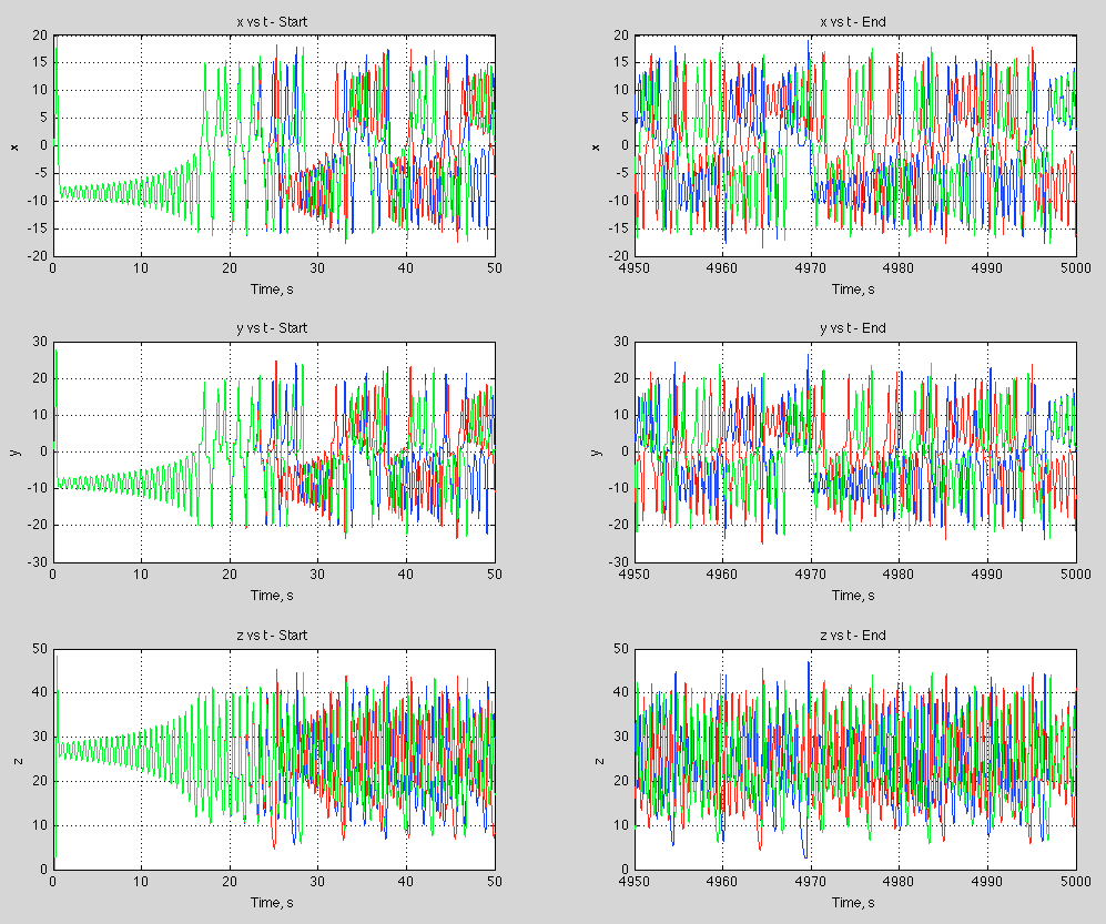
Figure 2 – click to expand – initial conditions x,y,z = 0, 1, 0; 0, 1.001, 0; 0, 1.002, 0
We can see that quite early on the two conditions diverge, and 5000 seconds later the system still exhibits similar “non-periodic” characteristics.
For interest let’s zoom in on just over 10 seconds of ‘x’ near the start and end:
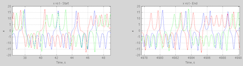
Figure 3
Going back to an important point from the first post, some chaotic systems will have predictable statistics even if the actual state at any future time is impossible to determine (due to uncertainty over the initial conditions).
So we’ll take a look at the statistics via a running average – click to expand:
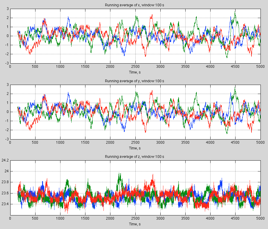
Figure 4 – click to expand
Two things stand out – first of all the running average over more than 100 “oscillations” still shows a large amount of variability. So at any one time, if we were to calculate the average from our current and historical experience we could easily end up calculating a value that was far from the “long term average”. Second – the “short term” average, if we can call it that, shows large variation at any given time between our slightly divergent initial conditions.
So we might believe – and be correct – that the long term statistics of slightly different initial conditions are identical, yet be fooled in practice.
Of course, surely it sorts itself out over a longer time scale?
I ran the same simulation (with just the first two starting conditions) for 25,000 seconds and then used a filter window of 1,000 seconds – click to expand:
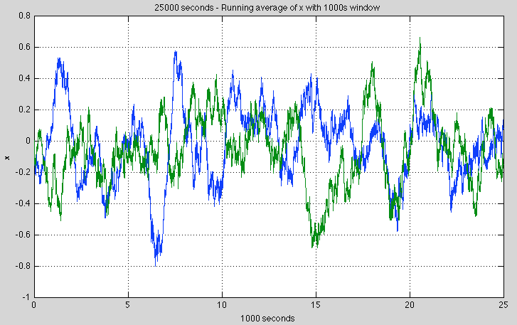
Figure 5 – click to expand
The total variability is less, but we have a similar problem – it’s just lower in magnitude. Again we see that the statistics of two slightly different initial conditions – if we were to view them by the running average at any one time – are likely to be different even over this much longer time frame.
From this 25,000 second simulation:
- take 10,000 random samples each of 25 second length and plot a histogram of the means of each sample (the sample means)
- same again for 100 seconds
- same again for 500 seconds
- same again for 3,000 seconds
Repeat for the data from the other initial condition.
Here is the result:
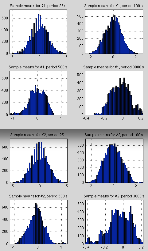
Figure 6
To make it easier to see, here is the difference between the two sets of histograms, normalized by the maximum value in each set:
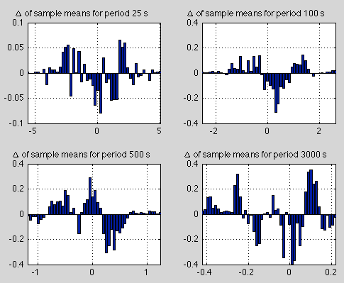
Figure 7
This is a different way of viewing what we saw in figures 4 & 5.
The spread of sample means shrinks as we increase the time period but the difference between the two data sets doesn’t seem to disappear (note 2).
Attractors and Phase Space
The above plots show how variables change with time. There’s another way to view the evolution of system dynamics and that is by “phase space”. It’s a name for a different kind of plot.
So instead of plotting x vs time, y vs time and z vs time – let’s plot x vs y vs z – click to expand:

Figure 8 – Click to expand – the colors blue, red & green represent the same initial conditions as in figure 2
Without some dynamic animation we can’t now tell how fast the system evolves. But we learn something else that turns out to be quite amazing. The system always end up on the same “phase space”. Perhaps that doesn’t seem amazing yet..
Figure 7 was with three initial conditions that are almost identical. Let’s look at three initial conditions that are very different: x,y,z = 0, 1, 0; 5, 5, 5; 20, 8, 1:
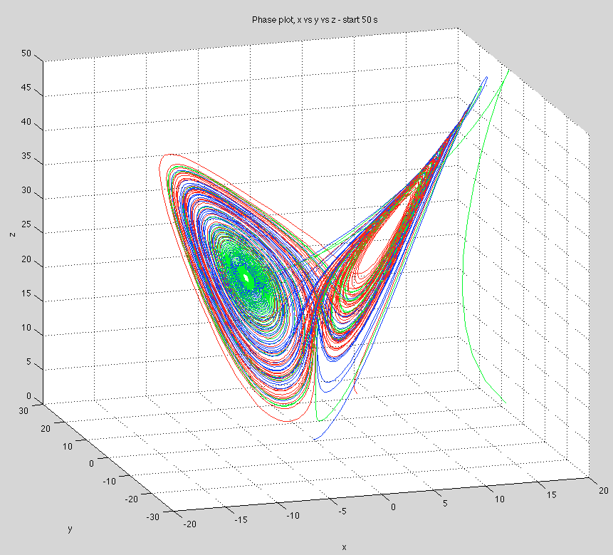
Figure 9 – Click to expand
Here’s an example (similar to figure 7) from Strogatz – a set of 10,000 closely separated initial conditions and how they separate at 3, 6, 9 and 15 seconds. The two key points:
- the fast separation of initial conditions
- the long term position of any of the initial conditions is still on the “attractor”
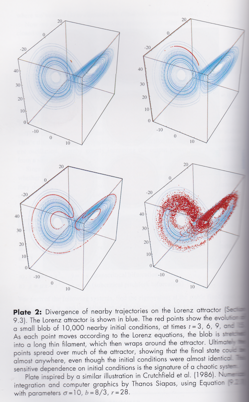
From Strogatz 1994
Figure 10
A dynamic visualization on Youtube with 500,000 initial conditions:
Figure 11
There’s lot of theory around all of this as you might expect. But in brief, in a “dissipative system” the “phase volume” contracts exponentially to zero. Yet for the Lorenz system somehow it doesn’t quite manage that. Instead, there are an infinite number of 2-d surfaces. Or something. For the sake of a not overly complex discussion a wide range of initial conditions ends up on something very close to a 2-d surface.
This is known as a strange attractor. And the Lorenz strange attractor looks like a butterfly.
Conclusion
Lorenz 1963 reduced convective flow (e.g., heating an atmosphere from the bottom) to a simple set of equations. Obviously these equations are a massively over-simplified version of anything like the real atmosphere. Yet, even with this very simple set of equations we find chaotic behavior.
Chaotic behavior in this example means:
- very small differences get amplified extremely quickly so that no matter how much you increase your knowledge of your starting conditions it doesn’t help much (note 3)
- starting conditions within certain boundaries will always end up within “attractor” boundaries, even though there might be non-periodic oscillations around this attractor
- the long term (infinite) statistics can be deterministic but over any “smaller” time period the statistics can be highly variable
Articles in the Series
Natural Variability and Chaos – One – Introduction
Natural Variability and Chaos – Two – Lorenz 1963
Natural Variability and Chaos – Three – Attribution & Fingerprints
Natural Variability and Chaos – Four – The Thirty Year Myth
Natural Variability and Chaos – Five – Why Should Observations match Models?
Natural Variability and Chaos – Six – El Nino
Natural Variability and Chaos – Seven – Attribution & Fingerprints Or Shadows?
Natural Variability and Chaos – Eight – Abrupt Change
References
Deterministic nonperiodic flow, EN Lorenz, Journal of the Atmospheric Sciences (1963)
Chaos: From Simple Models to Complex Systems, Cencini, Cecconi & Vulpiani, Series on Advances in Statistical Mechanics – Vol. 17 (2010)
Non Linear Dynamics and Chaos, Steven H. Strogatz, Perseus Books (1994)
Notes
Note 1: The Lorenz equations:
dx/dt = σ (y-x)
dy/dt = rx – y – xz
dz/dt = xy – bz
where
x = intensity of convection
y = temperature difference between ascending and descending currents
z = devision of temperature from a linear profile
σ = Prandtl number, ratio of momentum diffusivity to thermal diffusivity
r = Rayleigh number
b = “another parameter”
And the “classic parameters” are σ=10, b = 8/3, r = 28
Note 2: Lorenz 1963 has over 13,000 citations so I haven’t been able to find out if this system of equations is transitive or intransitive. Running Matlab on a home Mac reaches some limitations and I maxed out at 25,000 second simulations mapped onto a 0.01 second time step.
However, I’m not trying to prove anything specifically about the Lorenz 1963 equations, more illustrating some important characteristics of chaotic systems
Note 3: Small differences in initial conditions grow exponentially, until we reach the limits of the attractor. So it’s easy to show the “benefit” of more accurate data on initial conditions.
If we increase our precision on initial conditions by 1,000,000 times the increase in prediction time is a massive 2½ times longer.


[…] Does the surface temperature change with “back radiation”? Kramm vs Gerlich Natural Variability and Chaos – Two – Lorenz 1963 […]
If more CO2 in the atmosphere of the transport resistance increases (the net heat transfer remains substantially constant), and consequently rises the temperature difference between top and bottom. This increase in the temperature difference is distributed over a temperature increase at the surface and a decrease in temperature above – and in such a way that the total radiation remains constant into space through the atmospheric windows more intensity comes into space from the surface, from above – because colder – less emitted into space. The transport resistance can be described differently – eg with the net radiation as the difference between the upward radiation and back radiation. In this description, is more transportation resistance is more back radiation.
My problem with the deterministic chaos has always been that many of the results are highly dependent of the determinism at a very high level of accuracy, while few of the applications where the theory is used are deterministic in the same way. Another related issue is that the quantitative importance of the results depends also on the structure of the equations. In all typical examples there either are only very few variables or the set of equations can be written in a form, where a small number of equations controls the main behavior.
Adding even weak stochasticity to the set of equations might have an essential influence on the outcome from equations of the simple problem being discussed smoothening probably the averages over long enough averaging periods. At some point the results would not show any dependence on initial conditions any more. Some weak stochasticity might leave the Figure 4 above almost unchanged, but reduce essentially variability seen in Figure 5. The shape of the attractor would not change much in that case, but the way different parts of the attractor get populated might be very different.
When we consider the atmosphere or the whole Earth system the effectively stochastic contribution to the behavior is likely to be strong. The total number of variables is extremely large, infinite in continuum idealizations, some factor times the number of molecules or atoms for the discrete case.
What’s left and where from the deterministic chaos in the real Earth system?
The Earth system is chaotic. but not deterministic. Some subsystems or dynamic modes may follow at an useful level equations of some determistically chaotic model. Large scale ocean circulation might be an example, but I don’t think we have much evidence for that.
On a lighter note I was scanning back through the article looking for the inevitable typos and ouch.. take a look at figure 11 as it sits there with my comment underneath: “And the Lorenz strange attractor looks like a butterfly.” – er, no, in that youtube snapshot it looks like something quite disturbing..
SoD,
Very nice explanation. One of the things that is interesting to me is that chaotic systems are so resistant to improved accuracy of initial conditions; no matter how precisely the initial conditions are described, the system quickly diverges into unpredictability. For fluid flow, the equations themselves are demonstrably wrong, since the fluid is considered a continuum, when in reality it is a huge ensemble of molecules undergoing constant random motion and impacts. Treating it mathematically as a continuum introduces inevitable (tiny) error.
If you introduce a very small random error at each step in the iterative calculations, does the behavior evolve in the same way? I suspect the system may not “stay on the attractor”.
stevefitzpatrick,
I will be taking a look at adding random error (noise).
But it revolves around the attractor – otherwise there would be no gas laws.
SOD: How do I translate what I have seen in this post into “the real world of climate”. We have perhaps 6 to 10 decades of historic temperature data that is relatively unperturbed by anthropogenic GHGs and minimally perturbed by volcanoes and solar variation. Hoping to demonstrate “significant warming” in recent decades, I take the mean and standard deviation of the temperature data and calculate a 95% confidence interval. Does the fact that climate may be chaotic change how I would do or interpret such an analysis? I suspect that I need to ask if the data is stationary, auto-correlated, and normally-distributed.
If you repeated the above experiments a large number of times, would you expect that the mean would lie within twice the standard error of the mean from the first one experiment about 95% of the time?
Frank,
Probably (which, by the way, rules out I(1) or I(2) behavior in spite of what some econometricians think), definitely, dunno. The tests for auto-correlation assume that the underlying noise is normally distributed. Fractionally integrated noise is still stationary, but throws an additional monkey wrench into the works. Assuming an i.i.d. model ( independent, identically distributed) to calculate the standard deviation will undoubtedly underestimate the confidence limits.
Frank,
I don’t know.
Statistical significance is a mystery to me once we move from the world of throwing dice, pulling playing cards, or concocted AR(1) processes. You seem to have to know the things about your system you don’t know to calculate significance. I’ve seen the various tests. They give you some clues..
If we put your question in the context of the Lorenz 1963 system, it’s easy to have a flawed knowledge of the statistical characteristics of your system if you haven’t viewed a sufficiently long time period.
I’ve just starting building a simple model which will attempt to illustrate something a bit more like the climate, and the particular parameters we are all interested in in the climate. Might be ambitious, we will see..
The work you did for this post traveled part of the way towards providing an answer for the Lorentz system.
You wrote: “it’s easy to have a flawed knowledge of the statistical characteristics of your [chaotic] system if you haven’t viewed a sufficiently long time period.”
Lorentz expresses the same idea in terms of climate change: “Imagine for the moment a scenario in which we have traveled to a new location, with whose weather we are unfamiliar. For the first ten days or so the maximum temperature varies between 5 and 15 degC. Suddenly, on two successive days, it exceeds 25 degC. Do we on the second warm day, or perhaps the first, conclude that somebody or something is tampering with the weather? … Consider now a second scenario where a succession of ten or more decades without extreme global-averge temperature is followed by two decades with decidedly higher averages … Does this scenario really differ from the previous one? … Certainly no observations have told us that decadal-mean temperatures are nearly constant under constant external influences.
Click to access Chaos_spontaneous_greenhouse_1991.pdf
Frank’s quote of Lorenz above is an example of considering time scales. He suggests a rule that applies to a day, also applies to a period of 3650 days. If a day’s weather is argued to be noise, why not a decade’s weather?
Ragnaar: Lorenz wrote this paper about the time of the first IPCC report, after roughly one decade of rapid warming and speculated about what we would be able to conclude in 2000 if warming continued unabated for the 1990’s. He said that we didn’t have enough decades of temperature data to expect a confident statistical assessment about the meaning of one or two decades of strong warming. However, he believed that climate models could be used assess significance of warming – but only if the models hadn’t been tuned to match the historical record.
Here’s 3 diagrams of a bistable system, both wings of the Lorenz butterfly:

In the 1st diagram the prediction seems easy as we are on a trajectory to switch attractors. The 2nd diagram has a good chance of not switching attractors. The 3rd diagram is the most difficult to predict with about an equal chance of being on either attractor.
A question is, does nature do such things? The diagram could also represent weather forecasts with one attractor being rain and the other no rain. So perhaps nature can be modeled as such.
Here’s a diagram I found quite helpful:

Each image can said to be roughly, lots of rain or not. The possibilities are, this or that. The two attractors.
I deal with the tropopause and use the data of 47 years from the DWD. By the weather chaos there will be deviations from the trend. These deviations I once subjected to the Shapiro-Wilk test. The numerical value of the Shapiro-Wilk test is such a thing as the correlation coefficient between a normal distribution and the observed distribution. Full correlation is 1, the normal distribution is according to the central limit theorem result if many independent events leading to the observation. For comparison, I once used a Student distribution of 47 observations. In the Student distribution of the Shapiro-Wilk Tes returns the value 0.9966. The observations
of the temperature gradient deliver 0.9525
the pressure curve deliver 0.9831 and
the column pressure of CO2 0.9833
This has given a very high level of significance for the assumptions, that the deviations from the trend resulting from normal distributions.
The Shapiro-Wilk test is considered very powerful test.
Comments, corrections or criticisms would be appreciated on this paper under review:
Click to access Preprint_Solar_Energy.pdf
On another page I asked:
This is the graph in question:
Science, spirituality and religion seemed to be moving toward a common conclusion before 1946.
[moderator note – rest of comment snipped – this is a science blog, and comments need to stay on topic which is on science]
Nice post, and I will look forward to your future posts about how all this is related to climate. One thing that’s interesting about chaotic systems like the Lorenz attractor is the fact we can glean anything correct at all from computer calculations. There is always propagation of error in a numerical solution to an ODE, and with chaotic systems that show sensitivity to initial conditions, why don’t the numerical errors cascade into something that makes the solution useless for understanding the attractor, or the statistical properties of trajectories? I don’t know if this is well understood for the Lorenz system. There is something called the “shadowing lemma” that says essentially that numerical approximations are good enough for a certain type of strange attractor (“hyperbolic” attractors, see http://en.wikipedia.org/wiki/Shadowing_lemma). Not being an expert, I don’t know whether the Lorenz attractor (or other types of attractors that might show up in weather modeling) falls into that category.
A simpler example where you can see that numerical approximations predict the correct statistics, regardless of computing errors, is the logistic map x -> 4*x*(1-x). If you iterate this on the interval [0,1], you get a chaotic system, but one that is not too hard to analyze mathematically. You can explicitly calculate the distribution of a chaotic dense orbit as it fills up the interval [0,1] and verify that a numerical simulation gives the same distribution.
In my dynamical systems class, I learned that the Lorenz system actually having a strange attractor (as opposed to a ton of closed loops that somehow combine to look like the attractor) was only proven rigorously by mathematicians in the 90s!
[…] Part One and Part Two we had a look at chaotic systems and what that might mean for weather and climate. I was planning […]
[…] explained in Natural Variability and Chaos – Two – Lorenz 1963, there are two key points about a chaotic […]
[…] simple chaotic systems, like the Lorenz 1963 model. There is discussion of this in Part One and Part Two of this series. As some commenters have pointed out that doesn’t mean the climate works in […]
[…] One of the papers cited: Time Step Sensitivity of Nonlinear Atmospheric Models: Numerical Convergence, Truncation Error Growth, and Ensemble Design, Teixeira, Reynolds & Judd 2007 comments first on the Lorenz equations (see Natural Variability and Chaos – Two – Lorenz 1963): […]
“z = devision of temperature from a linear profile”
Sorry for a very basic question about the above definition of z … what does ‘devision’ mean? (Googling returns no result)
Richie,
Good question. It’s a typo, not a technical term. From the paper,
“The variable z is proportional to the distortion of the variable temperature profile from linearity”