In Part Four – The Thirty Year Myth we looked at the idea of climate as the “long term statistics” of weather. In one case, climate = statistics of weather, has been arbitrarily defined as over a 30 year period. In certain chaotic systems, “long term statistics” might be repeatable and reliable, but “long term” can’t be arbitrarily defined for convenience. Climate, when defined as predictable statistics of weather, might just as well be 100,000 years (note 1)
I’ve had a question about the current approach to climate models for some time and found it difficult to articulate. In reading Broad range of 2050 warming from an observationally constrained large climate model ensemble, Daniel Rowlands et al, Nature (2012) I found an explanation that helps me clarify my question.
This paper by Rowlands et al is similar in approach to that of Stainforth et al 2005 – the idea of much larger ensembles of climate models. The Stainforth paper was discussed in the comments of Models, On – and Off – the Catwalk – Part Four – Tuning & the Magic Behind the Scenes.
For new readers who want to understand a bit more about ensembles of models – take a look at Ensemble Forecasting.
Weather Forecasting
The basic idea behind ensembles for weather forecasts is that we have uncertainty about:
- the initial conditions – because observations are not perfect
- parameters in our model – because our understanding of the physics of weather is not perfect
So multiple simulations are run and the frequency of occurrence of, say, a severe storm tells us the probability that the severe storm will occur.
Given the short term nature of weather forecasts we can compare the frequency of occurrence of particular events with the % probability that our ensemble produced.
Let’s take an example to make it clear. Suppose the ensemble prediction of a severe storm in a certain area is 5%. The severe storm occurs. What can we make of the accuracy our prediction? Well, we can’t deduce anything from that event.
Why? Because we only had one occurrence.
Out of a 1000 future forecasts, the “5%ers” are going to occur 50 times – if we are right on the money with our probabilistic forecast. We need a lot of forecasts to be compared with a lot of results. Then we might find that 5%ers actually occur 20% of the time. Or only 1% of the time. Armed with this information we can a) try and improve our model because we know the deficiencies, and b) temper our ensemble forecast with our knowledge of how well it has historically predicted the 5%, 10%, 90% chances of occurrence.
This is exactly what currently happens with numerical weather prediction.
And if instead we run one simulation with our “best estimate” of initial conditions and parameters the results are not as good as the results from the ensemble.
Climate Forecasting
The idea behind ensembles of climate forecasts is subtly different. Initial conditions are no help with predicting the long term statistics (aka “climate”). But we still have a lot of uncertainty over model physics and parameterizations. So we run ensembles of simulations with slightly different physics/parameterizations (see note 2).
Assuming our model is a decent representation of climate, there are three important points:
- we need to know the timescale of “predictable statistics”, given constant “external” forcings (e.g. anthropogenic GHG changes)
- we need to cover the real range of possible parameterizations
- the results we get from ensembles can, at best, only ever give us the probabilities of outcomes over a given time period
Item 1 was discussed in the last article and I have not been able to find any discussion of this timescale in climate science papers (that doesn’t mean there aren’t any, hopefully someone can point me to a discussion of this topic).
Item 2 is something that I believe climate scientists are very interested in. The limitation has been, and still is, the computing power required.
Item 3 is what I want to discuss in this article, around the paper by Rowlands et al.
Rowlands et al 2012
In the latest generation of coupled atmosphere–ocean general circulation models (AOGCMs) contributing to the Coupled Model Intercomparison Project phase 3 (CMIP-3), uncertainties in key properties controlling the twenty-first century response to sustained anthropogenic greenhouse-gas forcing were not fully sampled, partially owing to a correlation between climate sensitivity and aerosol forcing, a tendency to overestimate ocean heat uptake and compensation between short-wave and long-wave feedbacks.
This complicates the interpretation of the ensemble spread as a direct uncertainty estimate, a point reflected in the fact that the ‘likely’ (>66% probability) uncertainty range on the transient response was explicitly subjectively assessed as −40% to +60% of the CMIP-3 ensemble mean for global-mean temperature in 2100, in the Intergovernmental Panel on Climate Change (IPCC) Fourth Assessment Report (AR4). The IPCC expert range was supported by a range of sources, including studies using pattern scaling, ensembles of intermediate-complexity models, and estimates of the strength of carbon-cycle feedbacks. From this evidence it is clear that the CMIP-3 ensemble, which represents a valuable expression of plausible responses consistent with our current ability to explore model structural uncertainties, fails to reflect the full range of uncertainties indicated by expert opinion and other methods..
..Perturbed-physics ensembles offer a systematic approach to quantify uncertainty in models of the climate system response to external forcing. Here we investigate uncertainties in the twenty-first century transient response in a multi-thousand-member ensemble of transient AOGCM simulations from 1920 to 2080 using HadCM3L, a version of the UK Met Office Unified Model, as part of the climateprediction.net British Broadcasting Corporation (BBC) climate change experiment (CCE). We generate ensemble members by perturbing the physics in the atmosphere, ocean and sulphur cycle components, with transient simulations driven by a set of natural forcing scenarios and the SRES A1B emissions scenario, and also control simulations to account for unforced model drifts.
[Emphasis added]. So this project runs a much larger ensemble than the CMIP3 models produced for AR4.
Figure 1 shows the evolution of global-mean surface temperatures in the ensemble (relative to 1961–1990), each coloured by the goodness-of-fit to observations of recent surface temperature changes, as detailed below.
From Rowlands et al 2012
The raw ensemble range (1.1–4.2 K around 2050), primarily driven by uncertainties in climate sensitivity (Supplementary Information), is potentially misleading because many ensemble members have an unrealistic response to the forcing over the past 50 years.
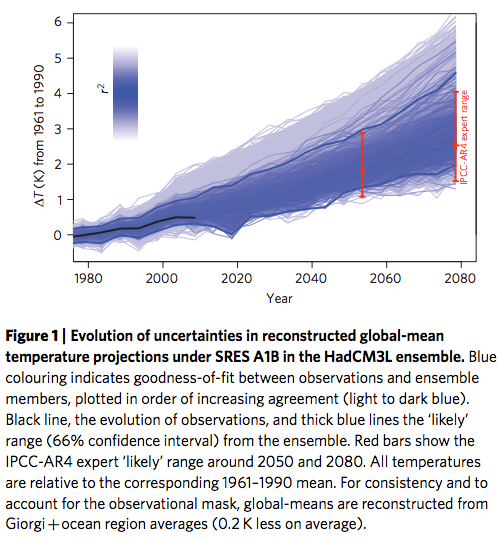
[Emphasis added]
And later in the paper:
..On the assumption that models that simulate past warming realistically are our best candidates for making estimates of the future..
So here’s my question:
If model simulations give us probabilistic forecasts of future climate, why are climate model simulations “compared” with the average of the last few years current “weather” – and those that don’t match up well are rejected or devalued?
It seems like an obvious thing to do, of course. But current averaged weather might be in the top 10% or the bottom 10% of probabilities. We have no way of knowing.
Let’s say that the current 10-year average of GMST = 13.7ºC (I haven’t looked up the right value).
Suppose for the given “external” conditions (solar output and latitudinal distribution, GHG concentration) the “climate” – i.e., the real long term statistics of weather – has an average of 14.5ºC, with a standard deviation for any 10-year period of 0.5ºC. That is, 95% of 10-year periods would lie inside 13.5 – 15.5ºC (2 std deviations).
If we run a lot of simulations (and they truly represent the climate) then of course we expect 5% to be outside 13.5 – 15.5ºC. If we reject that 5% as being “unrealistic of current climate”, we’ve arbitrarily and incorrectly reduced the spread of our ensemble.
If we assume that “current averaged weather” – at 13.7ºC – represents reality then we might bias our results even more, depending on the standard deviation that we calculate or assume. We might accept outliers of 13.0ºC because they are closer to our observable and reject good simulations of 15.0ºC because they are more than two standard deviations from our observable (note 3).
The whole point of running an ensemble of simulations is to find out what the spread is, given our current understanding of climate physics.
Let me give another example. One theory for initiation of El Nino is that its initiation is essentially a random process during certain favorable conditions. Now we might have a model that reproduced El Nino starting in 1998 and 10 models that reproduced El Nino starting in other years. Do we promote the El Nino model that “predicted in retrospect” 1998 and demote/reject the others? No. We might actually be rejecting better models. We would need to look at the statistics of lots of El Ninos to decide.
Kiehl 2007 & Knutti 2008
Here’s a couple of papers that don’t articulate the point of view of this article – however, they do comment on the uncertainties in parameter space from a different and yet related perspective.
First, Kiehl 2007:
Methods of testing these models with observations form an important part of model development and application. Over the past decade one such test is our ability to simulate the global anomaly in surface air temperature for the 20th century.. Climate model simulations of the 20th century can be compared in terms of their ability to reproduce this temperature record. This is now an established necessary test for global climate models.
Of course this is not a sufficient test of these models and other metrics should be used to test models..
..A review of the published literature on climate simulations of the 20th century indicates that a large number of fully coupled three dimensional climate models are able to simulate the global surface air temperature anomaly with a good degree of accuracy [Houghton et al., 2001]. For example all models simulate a global warming of 0.5 to 0.7°C over this time period to within 25% accuracy. This is viewed as a reassuring confirmation that models to first order capture the behavior of the physical climate system..
One curious aspect of this result is that it is also well known [Houghton et al., 2001] that the same models that agree in simulating the anomaly in surface air temperature differ significantly in their predicted climate sensitivity. The cited range in climate sensitivity from a wide collection of models is usually 1.5 to 4.5°C for a doubling of CO2, where most global climate models used for climate change studies vary by at least a factor of two in equilibrium sensitivity.
The question is: if climate models differ by a factor of 2 to 3 in their climate sensitivity, how can they all simulate the global temperature record with a reasonable degree of accuracy.
Second, Why are climate models reproducing the observed global surface warming so well? Knutti (2008):
The agreement between the CMIP3 simulated and observed 20th century warming is indeed remarkable. But do the current models simulate the right magnitude of warming for the right reasons? How much does the agreement really tell us?
Kiehl [2007] recently showed a correlation of climate sensitivity and total radiative forcing across an older set of models, suggesting that models with high sensitivity (strong feedbacks) avoid simulating too much warming by using a small net forcing (large negative aerosol forcing), and models with weak feedbacks can still simulate the observed warming with a larger forcing (weak aerosol forcing).
Climate sensitivity, aerosol forcing and ocean diffusivity are all uncertain and relatively poorly constrained from the observed surface warming and ocean heat uptake [e.g., Knutti et al., 2002; Forest et al., 2006]. Models differ because of their underlying assumptions and parameterizations, and it is plausible that choices are made based on the model’s ability to simulate observed trends..
..Models, therefore, simulate similar warming for different reasons, and it is unlikely that this effect would appear randomly. While it is impossible to know what decisions are made in the development process of each model, it seems plausible that choices are made based on agreement with observations as to what parameterizations are used, what forcing datasets are selected, or whether an uncertain forcing (e.g., mineral dust, land use change) or feedback (indirect aerosol effect) is incorporated or not.
..Second, the question is whether we should be worried about the correlation between total forcing and climate sensitivity. Schwartz et al. [2007] recently suggested that ‘‘the narrow range of modelled temperatures [in the CMIP3 models over the 20th century] gives a false sense of the certainty that has been achieved’’. Because of the good agreement between models and observations and compensating effects between climate sensitivity and radiative forcing (as shown here and by Kiehl [2007]) Schwartz et al. [2007] concluded that the CMIP3 models used in the most recent Intergovernmental Panel on Climate Change (IPCC) report [IPCC, 2007] ‘‘may give a false sense of their predictive capabilities’’.
Here I offer a different interpretation of the CMIP3 climate models. They constitute an ‘ensemble of opportunity’, they share biases, and probably do not sample the full range of uncertainty [Tebaldi and Knutti, 2007; Knutti et al., 2008]. The model development process is always open to influence, conscious or unconscious, from the participants’ knowledge of the observed changes. It is therefore neither surprising nor problematic that the simulated and observed trends in global temperature are in good agreement.
Conclusion
The idea that climate models should all reproduce global temperature anomalies over a 10-year or 20-year or 30-year time period, presupposes that we know:
a) climate, as the long term statistics of weather, can be reliably obtained over these time periods. Remember that with a simple chaotic system where we have “deity like powers” we can simulate the results and find the time period over which the statistics are reliable.
or
b) climate, as the 10-year (or 20-year or 30-year) statistics of weather is tightly constrained within a small range, to a high level of confidence, and therefore we can reject climate model simulations that fall outside this range.
Given that this Rowlands et al 2012 is attempting to better sample climate uncertainty by a larger ensemble it’s clear that this answer is not known in advance.
There are a lot of uncertainties in climate simulation. Constraining models to match the past may be under-sampling the actual range of climate variability.
Models are not reality. But if we accept that climate simulation is, at best, a probabilistic endeavor, then we must sample what the models produce, rather than throwing out results that don’t match the last 100 years of recorded temperature history.
Articles in the Series
Natural Variability and Chaos – One – Introduction
Natural Variability and Chaos – Two – Lorenz 1963
Natural Variability and Chaos – Three – Attribution & Fingerprints
Natural Variability and Chaos – Four – The Thirty Year Myth
Natural Variability and Chaos – Five – Why Should Observations match Models?
Natural Variability and Chaos – Six – El Nino
Natural Variability and Chaos – Seven – Attribution & Fingerprints Or Shadows?
Natural Variability and Chaos – Eight – Abrupt Change
References
Broad range of 2050 warming from an observationally constrained large climate model ensemble, Daniel Rowlands et al, Nature (2012) – free paper
Uncertainty in predictions of the climate response to rising levels of greenhouse gases, Stainforth et al, Nature (2005) – free paper
Why are climate models reproducing the observed global surface warming so well? Reto Knutti, GRL (2008) – free paper
Twentieth century climate model response and climate sensitivity, Jeffrey T Kiehl, GRL (2007) – free paper
Notes
Note 1: We are using the ideas that have been learnt from simple chaotic systems, like the Lorenz 1963 model. There is discussion of this in Part One and Part Two of this series. As some commenters have pointed out that doesn’t mean the climate works in the same way as these simple systems, it is much more complex.
The starting point is that weather is unpredictable. With modern numerical weather prediction (NWP) on current supercomputers we can get good forecasts 1 week ahead. But beyond that we might as well use the average value for that month in that location, measured over the last decade. It’s going to be better than a forecast from NWP.
The idea behind climate prediction is that even though picking the weather 8 weeks from now is a no-hoper, what we have learnt from simple chaotic systems is that the statistics of many chaotic systems can be reliably predicted.
Note 2: Models are run with different initial conditions as well. My only way of understanding this from a theoretical point of view (i.e., from anything other than a “practical” or “this is how we have always done it” approach) is to see different initial conditions as comparable to one model run over a much longer period.
That is, if climate is not an “initial value problem”, why are initial values changed in each ensemble member to assist climate model output? Running 10 simulations of the same model for 100 years, each with different initial conditions, should be equivalent to running one simulation for 1,000 years.
Well, that is not necessarily true because that 1,000 years might not sample the complete “attractor space”, which is the same point discussed in the last article.
Note 3: Models are usually compared to observations via temperature anomalies rather than via actual temperatures, see Models, On – and Off – the Catwalk – Part Four – Tuning & the Magic Behind the Scenes. The example was given for simplicity.


A kinda-sorta analogy is the use of stock or commodity technical analysis decision-making tools. One can pick any one of hundreds of tools, and then search the thousands of stocks or commodities and find one that matches the tool over a recent time period, like for a year or more. But anyone who has done much trading at all knows that has little or no predictive value for the future. Its just because you searched until you found a stock or commodity that matched the decision-making tool.
Spot on, SoD, and thank you very much for the Rowlands, et al 2012 paper! It, and your presentation, answers a question I long had about these ensemble model forecasts.
I don’t think *any* serious model should be rejected. All of ’em should be kept around and repeatedly retest. I think each of their scores of being correct should be kept as a posterior density at each moment. And, treating each model’s prediction of, say, global mean surface temperature, the estimates could be retrospectively smoothed, per http://www.lce.hut.fi/~ssarkka/course_k2011/pdf/handout7.pdf. That’s useful because it’s a sensible way of combining the effects of the repeated tests, one which avoids discussions of Bonferroni-like (repeated test) corrections or False Discovery Rate notions.
So, I get the impression — could be wrong — that the Rowlands, et al result is not widely appreciated in the climate literature? Why? And what are the implications for climate forecasts?
Robert Way gave at CA the link to a new article of Gavin Schmidt and Steven Sherwood: A practical philosophy of complex climate modelling
From there we can read comments supportive of what SoD wrote:
I haven’t yet read carefully the whole article. Thus this quote does not necessarily represent well all of it.
Part of the emphasis on (in)validating model predictions was the IPCC,
which in the 4th AR, boldly prognosticated:
“A temperature rise of about 0.2 °C per decade is projected for the next two decades for all SRES scenarios.”
Not sure if this was addressed or ignored in the 5th report.
But SOD, you are touching on something with which the IPCC 3rd AR agreed:
“In climate research and modelling, we should recognise that we are dealing with a coupled non-linear chaotic system,
and therefore that the
long-term prediction of future climate states is not possible.”
http://www.ipcc.ch/ipccreports/tar/wg1/505.htm
Climate Weenie,
You reminded me I was looking for these statements in the 3rd report (TAR) some time ago and couldn’t find them.
An expanded version of your extract above, from chapter 14, p771:
Í noticed that James Annan has just posted on his blog telling about criticism on the use of perturbed physics ensembles
http://julesandjames.blogspot.fi/2014/12/blueskiesresearchorguk-project-icad-and.html
I get the feeling this is not unlike playing Baccarat or some other game of chance. In other words, these people who were continually claiming “the science is settled” do not know what they’re doing – they’re just hoping they’re right.
Simply looking at the Vostok ice core record, it appears the return of the glaciers is overdue. The real concern is Global Ice. The extra particulates in the atmosphere now may be helping to delay their inevitable return.
How can it be *no* models are predicting Global Icing?
@brianrudze A mechanism which leads to extended CO2 drawdown, cooling, and so glaciation is a slowdown in tectonics, which impedes recycling of limestone formed from Urey reactions. I only mention that because, as comparisons are made with the past, I find it helpful to think of things like glaciation as less like beats of a clock than byproducts of Other Things Going On. No climate model includes tectonic effects, as far as I know, apart from steady state ones.
Also, to know whether I know what I am doing or not depends on my getting the uncertainty quantification correct. SoD, Rowland, et al, and Schmidt and Sherwood suggestion not everyone using ensembles is getting it correct. I’m happy about their observations, because they’ve settled some uncomfortable inconsistencies I’ve found in climate physics papers, including, but by no means limited to Fyfe, Gillett, and Zwiers.
I have not yet read in detail the BlueSkiesResearch blog post cited by Pekka, really rather the presentation by James Porter. I don’t know the mechanics of how PPE is done, but I would hope that in MME the parameters are varied over a range dictated by a reasonable prior for each of the parameter values, and for each of the models. The argument set up by James Empty Blog and BlueSkies seems to imply that PPE is parameter variation for limited models versus many models. I’ll need to come back to this after I’ve understood these links, but there could be practical, computational reasons why all these options are not done. Perhaps the links will explain.
(Further explanation.) Regarding the computational constraints … It is implicit in any weather and especially climate modeling campaign that the models need to do simulations at many, *many* times faster than the actual weather or climate develops, *especially* if an ensemble is to be run. Thus, I can imagine a tradeoff between fidelity of models which demands the code be complete but run slowly and models which are more approximate, but many versions of them can be run. At least in the USA, no climate model to my knowledge is run on adequate computing hardware. There is a plan to build such an exascale system, but it’s estimated to take 10 years to complete, with the software being developed in parallel. A number of references:
Click to access 1009.2416.pdf
Click to access NRC-Advancing-Climate-Modeling.pdf
Click to access olcf-requirements.pdf
http://scitation.aip.org/content/aip/magazine/physicstoday/article/60/1/10.1063/1.2709569
The presentation of James Porter does not contain much material relevant to this thread, only some short remarks. In his post James Annan refers also to earlier work by him and his collaborators, which are more relevant. Thus I see his post more as inspired by the presentation of Porter, but in substance based largely on his earlier work.
In Rownlands et al, the comparison between model output and observations is not based on a single number, say the global annual mean temperature, but on the similarity of the ‘spatio-temporal’ patterns. This means that what is compared is the spatially resolved evolution of temperature over the last decades. There is a rationale behind this, since these time evolving patterns contain information of the externally driven (GHG, aerosols, etc.) temperature evolution and of the internally generated (chaotic variability). If models were perfect, the simulated and observed external component should be equal. Models and the observed trajectory would then only deviate because of the presence in both of different realizations of the chaotic component (noise). However, at most only one model within the ensemble can be perfect, all others are wrong. If the externally forced signal of a model is very far away from the observed trajectory, it is not reasonable to consider them in equal terms with the others. It is thus reasonable, though debatable, to weight some models more strongly than others. Model trajectories that deviate from the observed trajectory are downgraded to obtain an estimation of the ranges of projected temperature for 2050. This is a standard approach within a Bayesian framework, in which prior assumptions are weighted by their likelihood assessed by comparing them to observations. Of course, it may happen that the observed trajectory is, by chance, not close to ‘centre of the distribution’, but this is the price that has to be paid if we want to ‘assimilate’ observations in our predictions.
A related, but also relevant question, is how the model ensemble is generated, i.e. with which joint probability distributions the model internal parameters are varied – in a Bayesian framework, the priors. Hargreaves and Annan have several papers on this as well.
eduardo,
It wasn’t my aim specifically to criticize the Rowlands et al paper. From one perspective it is very sensible what they have done.
It was the statement in the paper that helped my clarify my question (a question that I have had for some time).
If climate (=”statistics”) is predictable over 10 years, OR, climate is known to be tightly defined for a given external “forcing” then there is no argument with the approach.
If climate (“statistics”) is predictable over say 10,000 years (and climate is not known to be tightly defined for a given forcing) then the approach potentially has a very large flaw. And the climate models that are all selected/tuned because they match the last 150 years are under-sampling in a big way.
Can you comment on this? I believe you have published many papers(?)
Perhaps part of what has sparked some of my questions is the simplistic assertions in the blog world by let’s say “the consensus corner” that paints the “weather is an initial value problem, climate is a boundary value problem, QED!” picture.
But there is also a component of finding that the modeling world doesn’t seem, in practice, to believe that chaos is anything other than “a bit of noise”. Yet I read papers by co-authors of modeling papers who have written decent papers on chaos.
For example, this paper under discussion has Leonard A. Smith as a co-author, and he is also the author of two papers I’ve just been reading: Accountability and Error in Ensemble Forecasting, 1992; Identification and Prediction of Low Dimensional Dynamic Systems, 1996.
This is as much @SoD as it is @eduardo, whose perspective I fundamentally agree with.
But, I think, in this context and audience, here, we would like *not* an appeal to a slurry of references to previously published papers, as a set of links to code and data which explicate the arguments made in defense of the basic arguments.
What’s missing in even the classical Bayesian framework here, to my mind, is not that not only do *parameters* have priors, but there are sets of likelihood functions dictated by (climate) models which have weights and such. And if the posterior for a distribution of a critical parameter of interest is sought, such as expected economic output from a particular country, that expectation should be integrated over the set of possible likelihoods or models. Ensemble averages are, from my perspective, a poor man’s way of approaching that.
Also, I really don’t see at all why there should continue to be a gap between the “professional papers” in outlets like GRL and what SoD and Pekka and others here are seeking. Surely, there must be a set of code-embodied models, like Ray Pierrehumbert’s for his book, and data which advocate for these various opinions. Indeed, I’m beginning to embrace a new criterion for believing anything from physics or geophysics or population biology or meteorology or climate science: If the protagonist for a position cannot deliver typical models and data in the form of code and datasets to bolster their argument and allow their critics to play with it, I wonder about the robustness of the case.
Give us the models, And give us the corresponding code!
hypergeometric,
Model code and data is widely available.
For example, one of the climate models – CAM5 is available with extensive documentation:
You can download a copy of Description of the NCAR Community Atmosphere Model (CAM 5.0), a 280 page technical description of this model:
Many modeling groups have archived their data, e.g., the models that took part in CMIP5.
From An Overview of CMIP5 and the experiment design, Taylor, Stouffer & Meehl (2012):
The problem is that without access to a supercomputer you can’t do anything. This is also a challenge for climate scientists.
As an example, as seen in Ghosts of Climates Past – Twelve – GCM V – Ice Age Termination, a paper by Feng He et al produced a model of the last ice age termination. To me it seems – if this theory is true – that the ice age should have terminated much earlier. But no one has run the code for these earlier times:
I would like to use their model to falsify the theory. That is, the theory that “explains” why the last termination finished about 20 kyrs ago. But I can’t, because I don’t have a supercomputer.
I think this is the main limited factor.
Yeah, @SoD, that’s actually PRECISELY what I mean: If the minimal model suggested by researchers demands a supercomputer to run, then it is by chsracter not transparent. The models of Pierrehumbert inhospitable book don’t, and there must be comparable reduced models for the case each of these “community models” in specific situations demonstrates. I would argue that until such code and documentation is exposed, these are not fully scientific reports, no matter what the reviewers say.
In my comment above, when I said “..without access to a supercomputer you can’t do anything..” I meant “..without access to a supercomputer you can’t reproduce anything..”
As another note on availability of models, my understanding is that CAM5 can be downloaded.
I have NO IDEA where that word “inhospitable” came from with respect to Ray Pierrrehumbert’s wonderful, warm, engaging and interesting book, PRINCIPLES OF PLANETARY CLIMATE. I can only imagine a bad malfunction of the spelling checker on my Amazon Kindle Fire, which has been offline.
hypergeometric,
The problem is that there is no way around the supercomputing resource.
Imagine we said, “if we (outsiders) can’t run it, it’s not science” – then we would have no models.
Similarly, we have weather prediction which works well, saves lives, informs citizens, communities and governments – but is not accessible to the average person, even the average person armed with the necessary physics knowledge. Because we don’t have supercomputers.
Should we define weather prediction as “not fully scientific reports”?
The alternative is transparency.
For climate models it comes in the areas where we already have transparency:
– the model physics
– the model code
– the results (in archived data)
But also openness in how the models are developed.
This last area has perhaps been somewhat opaque to those outside the modeling community.
Papers like Mauritsen et al (2012) that we saw in Models, On – and Off – the Catwalk – Part Four – Tuning & the Magic Behind the Scenes are welcome improvements for people interested in climate science.
The problem with big models tends to be that they may be opaque also to the scientists who use them, not only to outsiders. In many fields big models are an invaluable tool, but a risky tool that may give spurious results, if used blindly. For this reason competent modelers and model users spend considerable effort to analyze the behavior of the model, and to figure out, what mechanisms within the model have been most important for the results that are of interest. That may involve running the model with different sets of parameters to see, how individual parameters change the results. That may also involve looking in great detail at internal variables of the model.
In many cases that kind of analysis of the model allows for constructing a much simpler model that reproduces the same effect, but is far too aggregated to explain much else. That kind of model may help others to understand the mechanism, but cannot usually prove that the explanation is true also for the real world and not only for the model.
Many scientific papers that are published based on models report on experimenting with models in the spirit of my first paragraph, but I would imagine that most of such analysis gets never reported in publications.
I got the impression that Hypergeometric proposed that modelers should more often present simplified models that have the mechanism they discuss in order to make their conclusions easier to assess.
Indeed, Ray Pierrehumbert keeps repeating in his textbook the theme “Big ideas come from simple models.”
Isaac Held wrote an excellent (and very readable for non-specialists) paper in 2005, The Gap between Simulation and Understanding in Climate Modeling on just this point:
By the way, for readers interested in the field, Isaac Held, who has been publishing great papers since the 1970s, has a blog which is well worth reading about atmospheric and ocean dynamics.
While in principle I agree with Held as quoted by SOD, I think the gap between “complex” models and theoretical understanding is probably very large. I would simply say as I’ve pointed out here that a very simplified form of the problem, the Navier-Stokes equations are ill-posed and we have a lot of trouble using these equations to get accurate answers for even remarkably simple problems over a broad range of Reynolds’ numbers. And we have pretty good data to use to calibrate the models for special classes of flows of interest.
The atmosphere is tremendously complex by comparison with very complex sub grid processes. Held himself showed on his blog that detailed models of convection gave totally different results depending on the size of the calculation domain. It just doesn’t pass the plausibility test that these models do anything very well. In fact, James Annan seems to say they lack skill at regional climate, which is what they seem to offer beyond simple conservation of energy models. They apparently do have skill at predicting the global temperature anomaly. OK, that’s a very very low bar.
I also believe that you will find a very large variation in the quality of the literature on these subjects. For Navier-Stokes many of the journals and certainly the AIAA conferences are selection bias factories. The fluid dynamics literature is more scientific and honest. I believe that this problem is present in climate science too. Most modelers do not understand even the basics of eddy viscosity models, but their models rely on them strongly. Gavin Schmidt for example didn’t realize that there were inherent errors in Reynolds averaging for non stationary flows. That’s OK and no one can know everything. But the more complex a modeling system, the less likely there is to be anyone who understands even the basics of all its parts.
I could be wrong about this, since I get my information by reading the documentation for the NCAR model and not from recent first hand experience using the models. But they are clearly based on the same principles as Navier-Stokes models and there are no miracles that occur as the problem gets more complex.
Not with respect to atmosphere, but for glacial flows, I remember a report that when a discretization of these was dropped from (if I remember correctly) cubic kilometer models to cubic meter models, whole ranges of realistic phenomena were revealed. This fed the argument that what many of these models need is far more computing power. Surely, it is possible to model many complicated phenomena (see FVCOM, which I am a little familiar with: http://fvcom.smast.umassd.edu/2014/01/10/3-outreach-march-11-2001-japan-tsunami/), demanding techniques like variable grids, but these need to be scaled up to the several forcings and boundaries which apply.
Sure, Navier-Stokes is unsolved, but, well, oceanography as a field tries to make do with models within parametric constraints of density, temperature, and viscosity. And turbulence isn’t completely out of reach for some of the ocean work, e.g., with respect to eddies. There’s a lot of work done at the mesoscale. My point is that predictability need not depend (to exaggerate) upon ab initio simulations from molecules.
See:
http://goo.gl/mDakXY
http://www.siam.org/news/news.php?id=2065
http://journals.ametsoc.org/doi/abs/10.1175/JAS4030.1
http://journals.ametsoc.org/doi/abs/10.1175/2010JPO4429.1
http://journals.ametsoc.org/doi/abs/10.1175/2009JPO4201.1
Even “chaos”, that conceptual Beetlejuice from the theory labs, is not insurmountable in many instances. Chaotic systems can be modeled and predicted, within limits, per Andy Fraser’s HIDDEN MARKOV MODELS AND DYNAMIC SYSTEMS, for example (http://www.fraserphysics.com/~andy/hmmdsbook/), but that discussion goes a place which I think quite unprofitable and in which I won’t any longer participate.
Yes, hyper, that’s all interesting research. In looking at it though, it looked qualitative in nature to me. You are looking at “phenomena” and showing complex interesting looking graphics. I did notice that for the ocean dynamics stuff, the Lyopanov exponent implied by the satellite data is a lot different.
What I look for are quantitative information and comparisons to data. There are also some important questions to answer about numerical consistency and repeatability that must be passed. If you use a much coarser or finer spatial grid, do you get a different result? If your time step is cut in half is there a significant difference? If you change your sub grid model a little, is there a big difference? If these tests are not passed, one must approach the results with caution. Also, do different numerical discretization schemes give different results? We see this a lot in fluid dynamics.
I do sometimes question all the colorful simulations and the money invested in them. Would we be better off trying to develop the cascade of models and theoretical understanding Held talks about?
David,
There are a lot of papers examining the effect of higher resolution on results.
Definitely with ice age simulation, rudimentary and “still getting out of the starting blocks” as it is. And with ocean simulation.
In looking at the development of models that attempted “ice age inception” as “perennial high latitude snow cover” – a necessary but not sufficient condition for starting an ice age – I found that the energy balance models could simulate perennial snow cover, then the basic GCMs that followed could not. More recently higher resolution GCMs can.
Oh good that’s solved then.. except.. maybe the next generation of higher resolution GCMs will show the opposite again.
With the massive limitation in computing resources it seems that research goes towards confirming theories rather than trying to falsify them.
The last ice age termination “proven” to be increasing high latitude solar insolation by a recent modeling study. Except the question is – why didn’t the even higher solar insolation at these latitudes in earlier years. The answer from the paper’s author – the funding was available for the study at 20kyrs.
Ocean simulation has a lot of problems due to the large grid size. Some regional studies with 1/10 degree grid sizes show bigger improvements.
So there’s definitely a strong interest in finding out what results we get from higher resolution. I expect this is a world away from the kind of resolution you are thinking about, but the computing capability just isn’t there.
For example, we are only just seeing ensemble simulations of 1000 members for periods of 100 years. And these are on an atmospheric grid size of something like 3 degrees – and needing flux correction.
When you have to “inject” momentum and energy (flux correction) to stop “unphysical” results developing I find the conclusions of the modeling studies to be extremely preliminary. Yet, the conclusions drawn from the era when models all had flux corrections were with “high confidence”.
Deser addresses some of this in her talk linked below. She and colleagues have diagnostics for climate models. There’s another talk on the same topic here https://www.simonsfoundation.org/multimedia/simons-foundation-lectures/science-of-climate/climate-projections-over-north-america-in-the-coming-decades/.
I’m no expert at this stuff, not like SoD and Pekka are, but I still get a feeling we’re talking past the problem. The “real worldline” is but one of a potentially infinite set of realizations it might have taken from any initialized hyperball, with the same boundary conditions. Good model ensembles (same model over many initializations, and then multiple models each over many initializations) can simulate those possible futures. Deser and colleagues has a technique for separating out this internal variability and, moreover, that variability is bounded, so eventually, the radiative forcing pulls away from the variability and is detectable. Detectability depends upon the response of interest, so temperature signals are stronger than precipitation. It’s not good at 50 years for anything, but at 100-200 years, it dominates.
hypergeometric,
There are big assumptions built into these techniques. I hope to demonstrate this in subsequent articles.
Okay, but are you proposing it’s possible to do Statistics without assumptions? I admit the size of the assumption may be somewhat subjective, but that is something that apparently you already have a well defined metric for.
hypergeometric,
The assumptions, the premises – they need to be defended.
As an example, going back to the earlier paper by Hegerl et al in Part Three, there is a statistical result but the required premise isn’t really clarified. Is it proven? Is it assumed?
I’ve followed up a lot of papers on Attribution referenced in AR5 (and references from those papers).
It still seems that some basics are assumed, not demonstrated, but maybe I haven’t understood the field at all..
More on this in due course.
Yes, SOD and hyper, I agree that increased grid resolution can be a good thing. Or at least it appears to show “realistic” looking “phenomena.” We see that in our simulations too. Better grid resolution often helps quantitative accuracy too. It also makes the problems harder to solve reliably. It may also increase the sensitivity to parameters because there is less numerical viscosity. It’s a mixed bag I think. What is unquestionably true is that it is something that is often easier to sell to money givers than more fundamental and riskier research. And it carries less risk for researchers too, since its usually relatively easy to do.
My main issue is seen in the statement “what we have learnt from simple chaotic systems is that the statistics of many chaotic systems can be reliably predicted.” I do not dispute some simple systems behave that way, however, there is no evidence that climate is such a system. Looking back at the best information we have of the Holocene, there have been significant variations larger than the present with different variations in all time scales (and all before human interference). Looking at the entire present Ice Age (about 3 million years) we have the glacial and interglacial cycles that were nearly periodic, but jumped from 40ky to 100ky spacings and had significantly different peak shapes and internal detail. Having some structure for a while does not imply long term trend beyond the limits imposed by the energy source and nature of the storage and release. You can likely project to a temperature band of plus and minus 2 degrees from present, 50 years from now, with a 95% probability, but not have much more than 50% probability which direction it will go.
Leonard,
I’m not claiming that the climate will follow these rules.
Lessons from chaotic systems are put forward for the climate, by climate science.
So as a starting point – if the principles learnt from simple chaotic systems are applied to climate I have questions about the application.
Leonard,
I agree that it is a coin flip as to whether the temperature will rise or fall over the next 20 or 50 years. If CO2 had any significant effect on global temperature the temperature could only rise given that its concentration in the atmosphere is rising monotonically.
The Stainforth (2005) paper seems to be available via http://www.climateprediction.net/wp-content/publications/nature_first_results.pdf
Thanks krmm, I updated the article with the link.
[…] are both due to the excellent discussion at the Science of Doom blog, so a hat tip to that community. Also, SoD reminded me of the insightful blog Dr Isaac Held writes, […]
“The researchers used a climate model, a so-called coupled ocean-atmosphere model, which they forced with the observed wind data of the last decades. For the abrupt changes during the 1970s and 1990s they calculated predictions which began a few months prior to the beginning of the observed climate shifts. The average of all predictions for both abrupt changes shows good agreement with the observed climate development in the Pacific. “The winds change the ocean currents which in turn affect the climate. In our study, we were able to identify and realistically reproduce the key processes for the two abrupt climate shifts,” says Prof. Latif. We have taken a major step forward in terms of short-term climate forecasting, especially with regard to the development of global warming. However, we are still miles away from any reliable answers to the question whether the coming winter in Germany will be rather warm or cold”. Prof. Latif cautions against too much optimism regarding short-term regional climate predictions: “Since the reliability of those predictions is still at about 50%, you might as well flip a coin”. http://www.geomar.de/en/news/article/klimavorhersagen-ueber-mehrere-jahre-moeglich/
Perturbed physics models evolve chaotically – with many divergent feasible solutions – as we are aware.
Although it does seem likely that individual realisations that haphazardly resemble one aspect of a system whose dynamics are fundamentally unrealisable at this time – may be less than informative.
It seems more solving the problem that can be solved – rather than the real but intractable problem.
Relevant to these series of posts, there’s a talk (I just listened to) by Clara Deser at NCAR,
and two papers she mentioned,
Click to access deser.internal_variab.climdyn10.pdf
Click to access thompson.internal_climate_variability_future.dec14.pdf
which address both internal variability, what you can expect to see in observations over short periods (generations of people, for instance), detectability and planning for climate outcomes, and limitations on the role of chaos in outcomes.
I’m curious about whether the problem here is well posed. For the policy maker the issue is “given the weather we’ve been having recently (aka the climate) what are the chances we’ll move to a different (hotter) state in the next 50 (say) years”.
Now it strikes me this is a much more constrained problem than the one being discussed here – particularly when you realise the future state we are worried about is the observed weather rather than some abstract notion of climate.
Adding to this are two other factors.
First the climates we have experienced over the last couple of millennia are limited – particularly when we put them in the context of our ability to measure them and the climate state that we are worried about in 50 years’ time.
Second the important thing for the policy maker is how best to manage the risks, so the premium is on understanding how the process will evolve, how the uncertainty will become constrained and what to keep an eye on.
Elsewhere I’ve suggested that forecasts from complex CGCMs aren’t likely to be the best tool to answer these questions (although they might help to understand the evolution of future weathers).
Seen in this light if one is using CGCMs I think one is particularly interested in those initialised to current weather and/or that reproduce it. Looking back in time the one thing we do know is the weather has memory (and so ipso facto does the climate) and it would be a mistake to throw that knowledge out with the bath water.
I also did not mean by any means to criticize this post. When reading your comment (‘..
f climate (=”statistics”) is predictable over 10 years, OR, climate is known to be tightly defined for a given external “forcing” then there is no argument with the approach.
If climate (“statistics”) is predictable over say 10,000 years (and climate is not known to be tightly defined for a given forcing) then the approach potentially has a very large flaw. And the climate models that are all selected/tuned because they match the last 150 years are under-sampling in a big way.
)
I have the feeling we may have an issue with definitions – and I agree here that not everyone attaches the same meaning to the concepts we are using here. So maybe that is partially one source of confusion or misunderstanding. My way of seeing this is as follows:
climate (probability distribution) is determined solely by the physical system (Earth + external forcings). Just for the sake of illustration we can generate a realization of today’s (say 2014) climate by running a climate simulation with constant forcing. Or alternatively we could imagine that the external forcings remain constant to their values in 2014 and we could observe the Earth for 10000 years under those conditions. But the concept ‘climate’ is not attached to a particular realization, it embodies a constant-in-time probability distribution. Note that this probability distribution can be very complex, also allowing for ‘abrupt climate change’ .For instance, if this probability distribution is bimodal and there are two possible stable states under the same external forcing. We see already here that the concept abrupt-climate change is ambiguous. Some persons use it to describe a realization that flips between two modes of one probability distribution , whereas others use it a change of the probability distribution itself because the external forcings may have changed.
According to one first definition, climate change would strictly denote a change in the probability distribution of the system, and thus it can only be caused by external forcings. However, you – and may others- may use the concept ‘climate change prediction’ to describe a trajectory (one realization of the probability distribution)) of the system caused by changes in the external forcings *and* determined by some initial conditions.
Within the first definition climate is tightly defined for a given forcing. Actually, given the physical system Earth, the external forcings completely determine the probability distribution called ‘climate’. I think this is the source of quite a few misunderstandings. I do not mean that this second definition is wrong, bit we have to be aware that it does not mean quite the same thing as he first definition.
Is climate change predictable over 10 years ? It depends. Within the first definition, I think it is. Not predictable would mean here that the probability distribution (not a particular trajectory) is extremely dependent on the external forcings. I think this is quite unlikely, even more so over 10 years. Within the second definition, it is probably not totally predictable. There will always be the part of potential variability attached to the initial conditions, which is not totally predictable.
I think that your question boils down to the following: what is the portion of potential variability that is caused by the external forcings and what is the portion of variability that is independent of the external forcings. In our parlance, what is the portion of forced to unforced (internal) variability. The answer depends on temporal and spatial scales. At regional and short time scales, the internal variability dominates; at long time and large spatial scales, the forced variability dominates. But where is the scale boundary (your question, in my interpretation) ? The answer also depends on the amplitude forcing variability. I can always predict that summers in New York will be colder that winters in New York, because the external forcing varies so much that the forced variability in NY always overwhelms the internal variability ( no all summers are equal). Thus, the probability distribution ‘New York summer’ is very different from ‘New York winters’. This difference is predictable. Within ‘New York summers’ , however, it is very difficult to predict which particular state will be realized.
The ‘consensus corner’ would probably argue that at multidecadal timescales the unforced portion is smaller than the forced portion, and thus climate change is quite predictable. I would be more cautious. My opinion, derived for instance from the paleoclimate record, is that our knowledge of internal variability is quite limited and in many stances clearly not correct. Climate models likely underestimate the internal portion.
Also, the concepts of probability distribution, realization, external forcings, predictability, etc., are solely our construct, which can be useful but also misleading. Nature does not know about any of those concepts.
I think this is the critical question for policy-making.
Clearly knowledge of internal variability is incomplete. But why, in your view, does it follow that models underestimate internal variability? Why shouldn’t we conclude that they overestimate it? Or get it about right? Or say, “we just don’t know”? Or all four, but under different conditions (as for different measures of climate, or for different regions)?
Also, I think it’s fraught to draw firm conclusions about the magnitude of internal variability in paleoclimate, because of the uncertainties in paleoclimate forcings. For example, we don’t have a tight estimate of present-day aerosol forcings (see http://www.ipcc.ch/pdf/assessment-report/ar4/wg1/ar4-wg1-chapter2.pdf FAQ 2.1, Fig.2), let alone ancient ones (which I think are estimated mostly by inference from ice-core sulfate and dust content).
Internal variability cannot be directly observed, since climate variability is always a mixture f forced and internal components. I agree with you that it is difficult to reach firm conclusions, and that is why I framed my comment as a rather a personal view, based on, say circumstantial, evidence. I will give here some examples. In the paper by Osborn on the evolution of the North Atlantic Oscillation through the 20th century as observed and simulated, it is concluded that the multidecadal variability of the NAO index- the long-term negative trend until 1970, the positive trend until 1995 and the negative trend thereafter, is not reproduced by models, not only is timing but its amplitude. This is based on observations, so that we do not have here the uncertainty stemming from proxy interpretation. Other example is the Medieval Warm Period, though perhaps not a global phenomenon, is clearly seen in many proxies in Eurasia. There is no clear explanation for the MWP, since the timing of the known external forcings – here essentially solar irradiance and volcanism – do not match the time of the MWP, peaking about 150 years later than temperatures do. Another example is the not so well known warm decades in the early 18th century in Europe, whose timing do not match the external forcings norare they reproduced by climate models driven by the known forcings.
Another example could be the recent hiatus in global temperatures. Some explanations for the hiatus is the increased heat flux into the ocean, which would be caused by internal variability (other explanations do involve external forcings tough). Most models do not reproduce a hiatus of this length and do so only when some climate models are artificially nudged with the ‘observed’ amplitude of internal variability in the Tropical SSTs for instance.
On the other hand, I am not aware of examples where models clearly overestimate the amplitude of internal modes of variations, like NAO, ENSO, PDO, etc.
The link from eduardo is:
Simulating the winter North Atlantic Oscillation: the roles of internal variability and greenhouse gas forcing, T. J. Osborn, Climate Dynamics (2004)
Just discovered this blog, enjoyed this post and comments very much. I’d like to re-ask something that I’ve asked elsewhere a number of times in the past: If current climate models do well at predicting the last century of surface temperatures, but have done much more poorly at predicting the first fifteen years of this century after the models were designed (obviously, correct me if this assumption is not true) – isn’t that in itself strong evidence that the models were tuned, overfitted, to the past century? This is the classical test for overfitting: a model that does much better on in-sample data than out-of-sample.
For instance, heat lost into the deep ocean is a currently popular explanation for the “pause” of the last ten/fifteen years. But we don’t even have ARGO data on the deep ocean for more than about five years! How did the models do well in the previous century, without incorporating data on deep ocean heat which we don’t even have?
Also: If the models need to be fixed (and all models do), how is anyone supposed to validate them? We get approximately _one_ new data point on average global surface temperatures per month! And no one claims that the models can predict anything more regionally specific than that.
Doesn’t mean we shouldn’t make models, but I don’t understand how we can use them for prediction if we can’t tell if they work at all.
‘Atmospheric and oceanic computational simulation models often successfully depict chaotic space–time patterns, flow phenomena, dynamical balances, and equilibrium distributions that mimic nature. This success is accomplished through necessary but nonunique choices for discrete algorithms, parameterizations, and coupled contributing processes that introduce structural instability into the model. Therefore, we should expect a degree of irreducible imprecision in quantitative correspondences with nature, even with plausibly formulated models and careful calibration (tuning) to several empirical measures. Where precision is an issue (e.g., in a climate forecast), only simulation ensembles made across systematically designed model families allow an estimate of the level of relevant irreducible imprecision…
Sensitive dependence and structural instability are humbling twin properties for chaotic dynamical systems, indicating limits about which kinds of questions are theoretically answerable. They echo other famous limitations on scientist’s expectations, namely the undecidability of some propositions within axiomatic mathematical systems (Gödel’s theorem) and the uncomputability of some algorithms due to excessive size of the calculation ‘
http://www.pnas.org/content/104/21/8709.full
To quote McWilliams from both the abstract and a footnote. James Hurrell and colleagues in an article in the Bulletin of the American Meteorological Society stated that the ‘global coupled atmosphere–ocean–land–cryosphere system exhibits a wide range of physical and dynamical phenomena with associated physical, biological, and chemical feedbacks that collectively result in a continuum of temporal and spatial variability. The traditional boundaries between weather and climate are, therefore, somewhat artificial. The large-scale climate, for instance, determines the environment for microscale (1 km or less) and mesoscale (from several kilometers to several hundred kilometers) processes that govern weather and local climate, and these small-scale processes likely have significant impacts on the evolution of the large-scale circulation (Fig. 1; derived from Meehl et al. 2001). The accurate representation of this continuum of variability in numerical models is, consequently, a challenging but essential goal. Fundamental barriers to advancing weather and climate prediction on time scales from days to years, as well as longstanding systematic errors in weather and climate models, are partly attributable to our limited understanding of and capability for simulating the complex, multiscale interactions intrinsic to atmospheric, oceanic, and cryospheric fluid motions.‘ http://journals.ametsoc.org/doi/pdf/10.1175/2009BAMS2752.1
Emphasis mine. It is partly grid resolution. Both problems require a whole lot more data and a whole lot more computing power. The weight of evidence is such that modellers are frantically revising their strategies. They have asked for an international climate computing centre and $5 billion (for 2000 times more computing power) to solve this new problem in climate forecasting. The monumental size of the task they have set themselves cannot be exaggerated.
Climate and models are chaotic but they are fundamentally different. Models have temporal chaos – calculation evolve a step at a time. Climate evolves in both space and time – spatio-temporal chaos. The ambition to encompass the latter with the former in the context of structural instability and sensitive dependence on the one hand and abrupt climate change on the other may be doomed to disappointment.
I think this comment simply reinforces my comment above. It is the utility of any model that counts, not its completeness however defined. We use arithmetic every day without bothering about Godel, we get up in the morning with plans for the day despite the inability to predict the future, and we use Newton’s laws despite (probably) knowing they don’t apply at nano and universal scales.
Just as the materials scientist grapples with the problems of detecting phenomena at smaller and smaller scales and needs to rely upon statistical characterisations to cover the unknown (and unknowable) so it is interesting to try and model the atmosphere in increasing detail.
But for practical purposes the policy maker wants to know what’s the temperature likely to be in 2050 plus or minus a few degrees. Spending more on increasingly sophisticated models and the grunt to run them on is unlikely to be the best investment to meet that policy imperative. We need to use models more appropriate to the task in hand.
miker613,
[Sorry it’s taken a few days to reply].
I’ve read a number of articles and a few papers to that effect (“current climate models ..have done much more poorly at predicting the first fifteen years of this century..”) but I haven’t examined it in detail.
This article is perhaps asking your question (about over-fitting) from a different perspective.
There is a common view on many blogs that models should match observations over a short time period. This is due to not really understanding what models can ever hope to achieve.
The problem is not at all easy to understand and it’s made more difficult by the polarized nature of the debate.
I have to admit that some time ago I misunderstood the “best-case climate modeling objective” as well. I’ve been helped by reading a lot on chaos and statistical fluid dynamic modeling (textbooks & papers, not blogs).
However, that has also produced more questions for me. Here the timescale is the question.
I have more questions than answers and I don’t have the answer to your question.
Being a bit boring, I think one fundamental aspect of the study of a technique (in this case multi-decadal modeling of climate using CFD models) is to consider its utility.
This is a meta model issue, it can’t be resolved by reference to the model itself it needs consideration of matters that lie beyond the model’s power to describe – just as the paradoxes such as Godel’s theorem cease to be an issue when considered in this light.
Formalising this is reasonably straight forward. You just define a utility function analogous to the truth function for formal logics. Note that this is different from the usual scientific tests that relate to how the model replicates other models, including observations (for the Solophists), although it will incorporate these considerations – utility and predictability often go hand-in-hand.
But one doesn’t really need to formalise this aspect to get benefit from thinking about these meta models. Just being aware of it helps tidy up disputes between protagonists.
The technician is fascinated by the structure of the models, how consistent they are etc etc. Others are looking for utility, but often with different utility functions in mind. There are different universes of discourse and it pays to get the rules of translation clear.
So it helps to be explicit about these differences and the limitations each protagonist faces if onle working in their own domain.
To bring it back to the subject in hand, among other things it teaches that a “best-case climate modeling objective” is a normative beast.
Comment from RichardS (relocated on request from the “Comments & Moderation” section):
First time here and novice. Appears to me that the IPCC, in pursuing global climate projections does a disservice. The people of this planet, IMHO, would be better off with regional projections. And wouldn’t regional forecasts lead to less computer demand and greater regional detail?
Regards,
Richard
Richard,
From what I understand, regional climate projections have much more uncertainty than global climate projections.
I expect to write about this in a future article.
Thank you. I look forward to that article. Been reading one of your articles from 2011 on water vapor feedback, which appears to conclude that geographic region plays a role. When that article was written there were limits in observational capabilities. Have there been any advances?
Speaking cynically, it is far easier to adjust a few parameters such as sensitivity to aerosols and hindcast 20th century warming in GMST than it is to climate change in several dozen regions correct at the same time with one set of parameters. Suppose two models project very different amounts of regional warming but similar global warming. The disagreement proves that at least one model is “wrong”. Does the agreement on global change have any scientific meaning?
I think this discussion would profit from broadening the concept of climate and climate change from GMST and change in GMST. Climate includes precipitation, especially regional and seasonal patterns in precipitation, which models should reproduce. Albedo/rSWR and TOA OLR are important aspects of climate. So are seasonal changes in regional temperature. For GHG-mediated climate change we have one “realization”. For seasonal climate change, we have up to a hundred realizations, but we don’t hear much about modeling seasonal change. Perhaps studying more than one observable can shed light on decadal natural variability.
A recent PNAS paper by Manabe shows that all models do a poor and inconsistent job of reproducing seasonal changes in OLR and rSWR observed from space in clear and cloudy skies by Erbe and Ceres.
Experimental work moves slowly. CERES and AIRS are pretty much state of the art but have been in operation for a while. People are always writing papers once there is a decade of experimental data. I don’t have anything significant to add but there have probably been over 1000 papers on water vapor in the last few years.
The article I was referring to can be found at this link. The difference between observed and modeled seasonal change in TOA LWR and reflected SWR. Figures 4 and 5 (which are worth posting) suggest that none of the 35 models is capable of reproducing all aspects of the seasonal changes observed by ERBE and CERES. Some models do a decent job with the clear sky LWR (combined water vapor plus lapse rate feedback), but clouds are a real problem. Reflected SWR (from snow in the NH winter) is another problem area.
These are the results from 10 realizations of seasonal change. FWIW, I find these discrepancies more important than the fact that models have modestly over-projected surface warming (by only about 25%) over the last 50 years.
http://www.pnas.org/content/110/19/7568.full
[…] « Natural Variability and Chaos – Five – Why Should Observations match Models? […]
The problem with the models you discuss has nothing to do with chaos. The problem for these models is that they are all based on a false hypothesis first stated in 1896 by Svante Arrhenius:
“The selective absorption of the atmosphere is……………..not exerted by the chief mass of the air, but in a high degree by aqueous vapor and carbonic acid, which are present in the air in small quantities.”
“Climate Science” is hopelessly corrupt given that so few of the practitioners care that their models can’t even explain the past, yet they presume to tell us what the global average temperature will be in 2100. Please stop trying to defend the indefensible. Richard Feynman explains:
“It doesn’t matter how beautiful your theory is, it doesn’t matter how smart you are. If it doesn’t agree with experiment, it’s wrong.”
gallopingcamel,
We can continue this part of the discussion in the location of your choosing (but not here):
On Uses of A 4 x 2: Arrhenius, The Last 15 years of Temperature History and Other Parodies – with the fact that Arrhenius is quite irrelevant in the field of radiative transfer.
Or The “Greenhouse” Effect Explained in Simple Terms – where like it says on the sticker, the basics, with links to relevant portions of the theory.
Or Theory and Experiment – Atmospheric Radiation – experimental values of total flux and spectra compared with the theory.
Or Understanding Atmospheric Radiation and the “Greenhouse” Effect – Part Six – The Equations – the equations of radiative transfer derived from fundamental physics.
Or another relevant article. I look forward to you presenting your ideas there.
Your arguments suggesting that it does not matter whether models correlate with observations are pure sophistry. You have lost contact with reality and the scientific method.
I will drop by again in a year or two but I am not hopeful that you can recover from this dreadful essay.
gallopingcamel,
It’s because you haven’t understood what happens in chaotic systems.
Have a read of Ensemble Forecasting where you can see that the successful weather forecasting approach is to work out frequencies of occurrence from “multiple model runs” (=ensembles), rather than to do one best forecast.
Because of the short time period of weather forecasting we can see that it works.
Can you explain why ensemble forecasting is used in weather forecasting?
Perhaps they have also lost contact with reality and the scientific method. Or perhaps they use it because there is no possibility of a deterministic forecast.
Following my sophistry a little, further abandoning reality and science, we might conclude that predicting the statistics of weather (climate) has similar problems.
Or we could ignore it.
gallopingcamel,
The statistics of the model have to match the statistics of the observations. But over what time period? 1 year, 10 years, 100 years, 1000 years, 10,000 years?
If you play around with a weather forecast until it matches last week’s weather you have an over-confident model. If you use it in the future it will not be as good as you think.
This is not in dispute in weather forecasting. The comparison is not between last week’s weather and last week’s forecast, it is the comparison between the statistics – how often did the 5% forecasts come true? How often did the 20% forecasts come true?
[…] And p. 1009 (note that we looked at Rowlands et al 2012 in Part Five – Why Should Observations match Models?): […]
SOD concluded with: “Models are not reality. But if we accept that climate simulation is, at best, a probabilistic endeavor, then we must sample what the models produce, rather than throwing out results that don’t match the last 100 years of recorded temperature history.
When ensembles of perturbed-parameter models are created, parameters are varied within a range that has been established by some sort of experiment. When initialized under a variety of conditions, the output from such ensembles represent the range of “future climates that are consistent with our understanding of the physics that govern climate”.
If we start with a single model, we can tune parameters one at a time and find a single value for that parameter that optimally reproduces some aspect of climate. Then we can tune another parameter. Eventually, from a small subset of parameter space, we find an optimum set of parameters from within the limited range of parameter space that we explore.
Why do conventional modelers believe (or act like they believe) that tuning produces an optimum model (to use in IPCC reports) while those modelers that work with large ensembles don’t want to discard any poorly performing models? It seems like the goal of ensembles should be to discard some regions of parameter space that perform poorly.
If some regions of parameter space hindcast excessive 20th century warming (1.5-2.5 degC and show low unforced variability), why are you against discarding them?
(You might want to argue that multi-decadal oscillations like the AMO or PDO exist (or worse, multi-centennial oscillations) and you may not have sampled the different states that are possible.)
Frank,
It’s a conundrum.
If – scenario A – the statistics of weather (=climate) are constant (for a given forcing) over say 30 years, then we should discard models that don’t match 30-year statistics.
That is, under scenario A, the job should be to find the parameters that match our observations. Parameters that give us results that don’t match observations are clearly not the correct parameters.
Nice and simple.
If – scenario B – the statistics of weather (=climate) are constant (for a given forcing) over say 100,000 years, then it would be a mistake to discard models that don’t match the last 30-year statistics.
That is, under scenario B, the job should be to use our modeling endeavors to discover the statistics of climate that we won’t be able to find by just observing the last 30 or 100 years of weather.
A bit tougher, because now we aren’t sure whether we are sampling “bad physics” parameter space as well as “good physics” parameter space. Or whether we are sampling climate statistics that haven’t yet been observed but are necessary to complete the picture of climate statistics.
The real problem is we don’t know whether scenario A or scenario B is correct.
Right now climate modelers, regardless of any philosophy they may have, act in practice as if scenario A is correct.
And because of the huge resources needed under scenario B in comparison with that available, it’s just not possible to practice climate modeling as if scenario B is correct.
However, just an opinion, if climate modeling computing resources suddenly went up 1 trillion times overnight, does anyone think that there wouldn’t be the immediate demand to run ensembles of 1M members each of 1M yrs. It’s only because of the practical limitations that current problems are attacked like they are.
SOD wrote: “The real problem is we don’t know whether scenario A or scenario B is correct.”
Agreed, but I think there are some situations where Scenario A is almost certainly the right answer. It is my impression that persistent weather patterns and unforced variability are mostly associated with SST anomalies and variations in vertical heat transport in the ocean. Stainforth’s ensemble used a slab ocean (60 m). Both the atmosphere and the mixed layer undergo massive seasonal changes outside the tropics and the ITCZ follows the sun north and south. With no upwelling, I doubt his output exhibits an ENSO or any other form of unforced variability. Is there any to show that the atmosphere plus mixed layer doesn’t follow Scenario A?
Scenario B isn’t a problem if the chaotic states that persist for longer than 30-years differ only modestly from each other. If GMST has varied only about 1 degC or less from phenomena like the PDO, AMO, LIA, MWP, RWP, etc. and if ECS is 3 degC or greater, we don’t need to pay too much attention to the Scenario B problem – it is just noise. IMO, another Maunder minimum or LIA or extended current hiatus won’t provide much help if ECS is high enough. Unfortunately, the chaotic behavior associated with ice ages and the chaotic behavior seen in Greenland during the last ice age suggests that unforced variability may have been unusually low over the last two millennia. The greatest climate change disaster on record since the last ice age may have been the desertification of the Sahara about five millennia ago; a great challenge for climate models. So I don’t disagree with your concern about scenario B from a scientific perspective.
There appears to be an interesting difference between a cooling and a warming planet. Surface warming produces a more stably stratified ocean; while surface cooling produces a less stably stratified ocean with more opportunities for tipping points that bring large amounts of cold deep water to the surface.
From a policy-making perspective, perhaps is makes sense to ignore scenario B. Long-term planning for any government on this planet is about 20 years. I like to imagine what today’s science might have warned policymakers about a century ago and whether policymakers could have intelligently invested a few percent of GDP back then to make the world a better place today. (Would they have warned that our cities would soon be buried in horsesh*t?) SLR seems to be one of the more intractable climate change problems, but if the current 1 inch/decade rate accelerates at 1 inch/decade/decade for the rest of the century, you only get 22 inches of SLR this century (about the IPCC’s central estimate). If that catastrophe is coming – and it isn’t on the horizon today – we should have many decades for adaptation.
All problems would not be solved even by infinite computational and analytic resources. At best we could determine the likelihoods of various outcomes for each model, but:
– We know that none of the models is a complete description of the Earth system. Thus we cannot expect that the model result are fully consistent with observations (even assuming no errors in the data). Rather we must allow for some differences and decide in some way, how to weigh each type of deviation.
– The available empirical data is very limited. Detailed data covers only a short period and earlier data is lacking in many ways. We have only one realization of the history, and the limitations of the data mean that splitting it to separate periods is of limited value for creating independent data sets. The possibility that the single history that we have is one that deviates significantly from the typical cannot be excluded.
From the above it follows that only models that deviate most strongly from the observations can be fully discarded in that imaginary situation.
In making predictions (or projections) based on analysis of models described above models that agree better with the observations should be given more weight. To what extent the most recent observations should have extra weight depends on the target period. For short term predictions agreement with recent history is more important than for long term predictions.
Pekka: We do have lots of empirical data about seasonal changes in climate. Models and ensembles of models could be evaluated for their ability to represent seasonal changes rather than decadal climate variability in terms of temperature anomalies.
Seasonal variability is one of many details that can be studied in addition to long term summary variables like the GMST.
A good climate model should describe reasonably well also seasonal variability and the most important spatial features including regional temperatures and precipitation as well as ocean circulation. Only then it’s possible to conclude that the model gets the dynamics right and has a change of describing feedbacks correctly. As long as some essential features are seriously wrong the model is not a valid physical model of the Earth system.
Overall energy balance can constrain at some level the model, but that’s not a strong constraint, and succeeding on that over some historical period does not prove that even this success is reached for the right reasons.
Pekka,
I’m not aware that any current climate model has any skill at the regional level. The idea that one can model regional climate with a finer resolution model with boundary conditions set by a coarser resolution model has been tried but has not been successful as far as I know.
DeWitt,
All GCMs have some skill as all tell that equator is warmer than poles and many other things correctly. Thus the question is not whether they have any skill but whether they have sufficient skill, and that depends on the requirements of the particular analysis.
Pekka,
I don’t consider that having the equator warmer than the poles demonstrates skill at the regional level. An extremely simple energy balance model with a rotating sphere exposed to sunlight has the equator warmer than the poles as long as the surface doesn’t have extremely high thermal conductivity. Skill means doing better than a simple model. For something as complex as a GCM, that should be a lot better.
DeWitt,
My purpose was to emphasize by the extreme example that the requirements depend on the particular goals of the study and that a model that’s badly deficient for one purpose may be useful for another. Concluding that requires, however, good justification.
More specifically it’s quite possible that a model has reasonable dynamical behavior, but fails in describing the precipitation in some important area due to some reason that’s understood. I don’t think that the problems are presently understood well enough. The example presented in the later post on abrupt change in a model calculation is a clear example on the deficient understanding of the model dynamics – and consequently also of the dynamics of the real Earth system.
Models are used for different things as Pekka notes.
If they are a surrogate lab in which we are testing behaviour of theoretical climates within sample we want the full range of responses once we have established the lab is fit-for-purpose. I just note that this latter process should use criteria that are established a priori.
If we want to forecast (out of sample) we are going to want models that validate out of sample and that model the earth’s historic weather. If I want to know what is going to happen in 2050-2100 I wouldn’t want to be using anything other than the family of models that get us to 2015 safe and sound.
After all a few constraints on the problem won’t be a bad thing.
Noting that all models have a mean rate of warming that exceeds that of the recent past and assuming that they are good enough to be useful in projecting the future, we can conclude that the natural variability has probably brought the temperature to a value less than the climatic expectation value. Thus the expected future behavior includes some warming from mean reversal on top of the warming from the trend. The autocorrelations of the internal variability processes determine the rate of the expected reversal to the mean.
My earlier comment that appropriate weighing of the model runs depends on the interval to the point of time for which the projection is presented was based on the above reasoning. For short intervals it’s important to get the initial temperature close to the correct value, for longer intervals the only thing that matters for the expectation values is the correct mean climate. In determining the correct mean climate the most recent years have no more weight that earlier years as long as the data is of the same quality. (The increasing forcing from CO2 does, however, affect the weight of later years in determining parameters connected to climate sensitivity.)
Pekka
With an underlying autoregressive process judged to be at an low extreme there will be a stagger upwards to compensate, but that will be encoded in any decent model. It would be a mistake to separately select in favour of those models when doing one’s projections because that would amplify the effect.
There is a little issue sitting in this about the separation between weather and climate on a global basis and how to do this in practice (discussed in one of the earlier threads). I’d be curious on your or anyone else view as to how many different global climates we have had in the last 2000 years and what they were. This helps to think about what the next different climate will be and what in fact we are projection. If you don’t know what you are projecting it becomes hard to validate. The problem is the lack of any recognizable boundaries in nature at the global level.
Also part of the point at issue is how you go about creating reliable models for projection purposes and then how to use them for projection. The risk in the current situation is that the models haven’t been properly validated out of sample and the rate of warming shown in the models is an artifact of the models rather than the real world. We are close to the point as I understand it where the hypothesis that we are just seeing the extreme of underlying natural variation as defined in the models is breaking down.
HAS,
Adding the effect twice would be an error, but what I had in mind is:
– In case of near term (like 5-10 years) prediction give more weight to model runs that happen to have a recent hiatus as well and that deviate downwards from other runs of the same model at the end of the historical period.
– In case of longer term projections (say 50 years) give equal weight to all model runs of the same model.
Thus what I discussed applies mainly to weighing the model runs of each model separately. How to weigh different models should depend on their overall success in describing historical data and in other tests of their validity.
DeWitt Payne
I’m going to take a look at regional forecasts in another article, because I see a fundamental problem – or maybe I just have a small question – with models being unable to forecast at a regional level. It’s along the lines of “if you can’t forecast the temperature in the Labrador Sea how will your AMOC be correct, and if your AMOC isn’t correct you will fail to model one of the most important millennial climate features.”
The non-linearity of climate in essence means that getting the location wrong isn’t something that just comes out in the GMST wash.
Well, that’s pretty much the article, but I was going to cut and paste some text and a few graphics from a paper or two to pad it out..
SoD,
Thanks. I needed that. Good thing I wasn’t drinking anything when I read that though or you’d owe me a keyboard.
Pekka wrote: “Noting that all models have a mean rate of warming that exceeds that of the recent past and assuming that they are good enough to be useful in projecting the future, we can conclude that the natural variability has probably brought the temperature to a value less than the climatic expectation value.”
I’d like to suggest a different conclusion: “Noting that all models have a mean rate of warming that exceeds that of the recent past” and noting that the models show low unforced variability, we can conclude that they are wrong about either climate sensitivity or unforced variability. If my conclusion is justified, can the models be good enough to be useful in projecting the future?
The “recent past” now includes from the last 1-4 decades (Otto 2013) and now the last 65 and 130 years (Lewis and Curry).
Frank,
On theoretical grounds it’s highly unlikely that the relationship between CO2 concentration and the GMST is highly non-linear as long as the changes in temperature are only a degree or two. Therefore the evidence for the effect I proposed is relatively strong.
I agree that all observations of temperatures of the latest years that fall below the mean trends of a model adds also some evidence that the model “runs too hot”, but this evidence accrues more slowly and must be considered as part of the overall evidence of all kind.
I commented above on the natural variability side of the issue.
What I don’t understand here is the suggestion we need CO2 & GMST to be highly non-linear for the separation between forcings and natural variation to be incorrectly modeled.
HAS,
By that I meant that it’s unlikely that the mean trend is significant with somewhat less CO2 or little lower temperatures, but goes rapidly to a very low value with more CO2 and slightly higher initial temperature.
That could be true, if the relationship where highly nonlinear in the direction of saturation of the warming influence of CO2.
Pekka: You noted that models were running hot and – assuming they made useful projections – concluded the problem must be natural variability. I noted that models don’t exhibit enough unforced variability for unforced variability to be a viable explanation. That leaves naturally-forced variability – solar and volcanic. Are you claiming the explanation lies here?
Frank,
You can replace “running too hot” by any other deviation from observations.
My general point is that comparing numerous model runs with the observations tells about two things:
(1) How good the models are.
(2) Which of the model runs happen to agree best with the recent observations.
Based on (1) we may judge that some of the models disagree too badly with the observations. Such models may be excluded from making projections. That test is based on all data without special emphasis on the most recent years.
Comparison (2) may be used to get better short term projections by weighing the runs based on recent agreement.
Why should observations match models? Because it is pleasing if a model matches observations.
It’s surprising how simple a climate model can be while both matching historic temperatures and making a fairly accurate 24-year hindcast from 1991, including the pause in warming that FAR(1990) and CMIP3(2007) did not predict :

Of course this was achieved top-down by curve-fitting, so sniff derisively if you must. The news (via Knutti) that even the CMIP3 crowd were tweaking one parameter down (aerosols) and another parameter up (ECS), thus all producing mutually contradictory hypotheses of climate parameter values despite their total output still matching history, simply shows that curve fitting is standard practice even at the top end of town.
But the test of any model, no matter how it is constructed, is how well it extrapolates beyond the training data set. Providing you judge it on 10-year averaged trends, I reckon a 24 year hindcast with RMS error of less than 0.04 Kelvin (as shown) is not so bad for a hybrid physical/statistical model that runs in a spreadsheet. It makes a few conjectures about water vapour and the Svensmark effect, but in this game who hasn’t?
This does not model *how* the climate operates, it has merely shown good performance as a phenomenological model of sea surface temperature over the most recent 150 years. The 64 year cycle of the AMO (incorrectly labelled PDO in this old screenshot) is the main contributor to its short term accuracy, though I am sure the cycle will not have a constant period in the coming decades.
Luckily SoD has provided the explanation for why this model is no worse than the top-dollar IPCC models: because no matter how far the model diverges from observation you can always claim the observations were an aggregation of statistically unlikely events and that the model shows the true underlying “strange attractor” which has had non-stationary “reality noise” unhelpfully superimposed on top of it in all observations. Nice escape clause there. But is it Science?
Why is there a secular trend in your sine wave? You can get quite a good fit to the temperature time series with a sine wave and an exponential. That fit does not predict declining future temperature.
Hi DeWitt,
Even a pure sine wave will appear to have a linear trend in it if you perform the regression between two points that are not a whole number of wavelengths apart. That’s how AMO, despite being a trendless oscillation, has contributed to the linear trend from 1900 to 2014.
Well I’m sure you know that a pure sine wave does not have a secular trend, so your conclusion about the above graph would then be…. what? 🙂
Svensmark. He was right. Solar magnetic activity went up mid century.
Leif has tried to convince everybody on WUWT that it didn’t happen, but the problem with his coverup attempt is that we have the sunspot counts, and the sunspots don’t lie.
(It’s also possible the amount of solar UV acting on ozone has had some climatic effect, which I don’t understand except to say that UV amount also changes over the solar cycles like cosmic ray shielding does, so my model may make a roughly accurate prediction for the wrong reasons.)
As solar magnetic activity declines over the next 50 years and the AMO cycle goes into the descending phase over the next 20 years then in total we should see a decline in world temperature between now and 2040.
It would not surprise me if I was wrong about this conjecture as I do not have the long experience all the climate scientists have. However I insist that the conditions to test the above hypothesis at 1:1 scale in vivo have not arisen until now, so all prior dismissal of these ideas could not have had an empirical basis. We are entering a very interesting time for climate science over the next 10 years as for the first time since the satellite era began the two factors I believe to be responsible for most of late 20th century warming are transitioning into a cooling effect, while of course CO2 continues to skyrocket exponentially. For the first time (ever) in climate science we will be able to gauge the relative strength of these 3 factors in altering sea surface temperature.
It’s just a shame that the Earth-Sun system only generates new climate data points at the rate of 1/30th of a measurement per year. I expect the politicians in Paris will not wait for the truth.
Sure you can have an apparent secular trend if you start and end out of phase. I’m asking why, when measured at the peak, the value decreases each cycle. Specifically, why is the peak near 2005 higher than the one near 2075?
Hi DeWitt,
I feel I should apologise as I have just realised that old screenshot did not have the definition of the Albedo(t) function displayed. However the obvious hint was in the title: “Simple Sunspot/Ocean/CO2 Climate Model”.
Obviously, the chart does not look like a pure sine wave because it is not a pure sine wave. So you are really asking what else is in the model aside from the sinusoidal ocean cycle and the CO2.
I have already advertised my exaltations for Svensmark’s theory and I am on that bandwagon at least until it either falls apart or I find something better. So I thought it was also obvious that cosmic ray-induced albedo modulation was the main cause of the undulation in cyclic temperature peaks. It is interesting, isn’t it, that you only need to suppose that history will repeat itself in order to explain most of the late 20th-century rise in temperature via natural causes.
It’s basically been a case of natural co-incidences. Just before the oceanic cycle had peaked in 1945 and began cooling, the solar activity increased from 1938 to 1964 and basically topped up the oceans with extra heat while they “should” have been cyclically cooling. Then that solar activity slowly decreased again over the next 44 years just as the 64 year oceanic cycle went back into warming phase in 1976. The solar activity increase cancelled out the ocean cooling for half an AMO cycle, leading to 90 years of warming from 1910. It’s funny that SoD is right about observations being a result of unlikely events… but perhaps not in the way he had supposed. 😉
I’ve assumed CO2 increases warm the ocean even though there is no observational evidence that it can do that directly via radiation. Therefore ongoing CO2 radiant forcing will increase temperatures above normal, but CO2 is a distant 3rd place in accounting for variance over the past century, after AMO and solar activity. You will notice that in the forecast by 2100 there is a significant 0.5 degree difference between the static CO2@1900 scenario and the industrial BAU scenario. Just because the IPCC’s attribution statement on the 20th century is false does not mean CO2 won’t make a significant difference in future. Knowing how much difference it makes is still important to formulating a wise response, in both mitigation and adaptation.
Ah, I still didn’t answer your specific question which was: “Specifically, why is the peak near 2005 higher than the one near 2075?”
Because most astrophysicists agree (!) that solar activity is forecast to decrease over this century and my model incorporates the causal link between solar activity and ocean temperature known from proxy studies such as Neff (cited above), Shaviv’s reconstruction, and recorded history (Maunder minimum/CET).
Andrew M wrote: “CO2 is a distant 3rd place in accounting for variance over the past century, after AMO and solar activity.” He also provided a link to a Roth and Joos paper reconstructing TSI from C14. The abstract includes this statement:
“A recently published solar activity–TSI relationship yields small changes in Holocene TSI of the order of 1 W m−2 with a Maunder Minimum irradiance reduction of 0.85 ± 0.16 W m−2.”
If my memory is correct, 1 W/m2 is the highest published value for the decrease in TSI during the Maunder Minimum and there are lower estimates.
Given that the forcing from GHGs is currently about 3 W/m2 and that solar changes in the past century appear to have been much less dramatic than the Maunder Minimum, I’m not sure why Andrew puts solar TSI ahead of GHGs.
There are other forms of “solar activity” besides TSI and they aren’t quantified in terms of W/m2 (like most forcing): 1) Fluctuations in higher energy radiation (UV and particle) emitted by the sun. Such fluctuations are observed during the solar cycle, which has a negligible impact on our climate. 2) Fluctuations in the strength of the solar magnetic field, which blocks cosmic rays. The C14 and Be10 records tell us nothing unusual happened to the solar magnetic field during the past century.
SOD has never discussed changes in solar activity. After reading ClimateDialogue and some other work on this subject, I was left with the impression that “big changes” in “solar activity” could be looming, but that they would be small compared with GHGs.
The amount of unforced variability the AMO has contributed to climate change during the instrument period depends on your preferred value for climate sensitivity. However, I’m not aware of any estimates that make the AMO the dominant player. Lewis and Curry (2014) calculate ECS and TCR by assuming that all warming between the same phase AMO (a 65 year period and a 130-year period) is due to forced variability and obtain remarkably low estimates for climate sensitivity. That analysis still leaves only a modest role for the unforced variability associated with the AMO – perhaps only a peak to trough amplitude of 0.2? degC. If one ignores the warming due to GHGs – which I don’t think is scientifically appropriate – and assumes that AMO causes the full dynamic range of climate change over the same period, the calculated amplitude will be much larger.
I wouldn’t say much larger unless you consider a factor of about two to be much larger. It’s easy enough to fit a 65 year period sine wave to the surface temperature record. IIRC, peak to trough is about 0.4°C. What’s left looks remarkably like what one would expect from ghg forcing without any significant effect of aerosols, or a nearly constant aerosol effect. A quick and dirty method is to use a 65 year moving average.
There may be a ~21 year periodic variation as well, which would be about what one would expect from the solar cycle. Paul_K did a post or two on this at The Blackboard a while back.
Paul_K’s articles are here and here. In his fit, the contribution from the sum of the 21 and 61 year cycles was about 0.3°C peak to trough.
DeWitt: Thanks for the links. Paul_K is often brilliant, but I don’t think science makes much progress through curve-fitting exercises that select one hypothesis from an infinite number of possibilities. I prefer to pick and test one hypothesis at a time.
The original paper characterizing a roughly 65-year AMO showed a consistent signal localized in and around the Atlantic. A sensible mechanism for producing the AMO exists – variation in the MOC – but we lack a long record of changes in the MOC.
Like the AMO, the ENSO arises from changes in ocean currents (and winds). ENSO teaches me that the amplitude and period of such oscillations can be highly irregular. The two cycles of AMO found in the instrumental record could be similar by chance and not typical of how the AMO normally behaves.
Before putting the AMO in a model, I want evidence for more than two cycles. I conducted my own “experiment” and looked at the Central England Temperature record, finding a paper with evidence supporting several more cycles of the AMO. So the AMO HYPOTHESIS has passed ONE test. I’d sure like to see more paleoclimate evidence from the regions that recorded the last two cycles of the AMO (and not two other papers I found with a 65-year period on the other side of the world. Such papers merely prove that Fourier transforms find things by chance no matter what the statistical analysis I don’t understand tells us about the likelihood of finding a fit by chance.)
The paper that discovered the AMO scanned the whole planet for similar local phenomena and didn’t find anything around 21 years. Local phenomena can be driven by oscillations in ocean currents, but global phenomena might originate outside the planet. The solar cycle formally repeats every 22 years, but everything we associate with “solar activity” has an 11-year period. Without any confirmation that a 21-year cycle exists, I don’t want it in my model
Paul’s residual SURE doesn’t look much like GHG forcing to me (but I skimmed this part). If Paul_K wants to attribute this signal to GHG’s, he should use the GHG forcing record in place of the SURE (with or without aerosol forcing, which could be greatly exaggerated.) There is good evidence for the hypothesis that GHGs should have some effect on climate.
I couldn’t find amplitudes in Paul_K’s post, but Loehle and Scafetta (2011) covered somewhat the same ground. The peak to trough amplitude for their 60-year cycle was 0.24 degC and the 20-year cycle was about 0.08 degC.
Click to access 1206.5845.pdf
Whether or not my perspective is the appropriate one, the AMO still appears to be a smaller influence than GHGs. The influence of GHGs will grow in the future.
Frank,
Even if the periodicity of the AMO is in doubt, it’s a testable hypothesis. We should see within the next decade or less if the AMO starts to go negative and temperature agrees with the extrapolation rather than the models. There will be other consequences as well. Arctic sea ice will, IMO, be the canary in the mine. The rapid death spiral folks already have egg on their faces.
Frank said:
> > “I’m not sure why Andrew puts solar TSI ahead of GHGs.”
Frank, I never mentioned TSI, and you certainly did not quote any words of mine to the same effect, so you’re fighting a strawman there.
I referred to that Roth + Joos paper only because they expect solar activity to decrease; I could have referenced NASA’s predictions or Abdusamatov’s predictions and that would have the same value to my model, which is that the activity will decrease, with commensurate change in heliospheric magnetic field, UV, and TSI. It’s the magnetic field that is the important part for the Svensmark effect.
Frank said:
> > “The C14 and Be10 records tell us nothing unusual happened to the solar magnetic field during the past century.”
That was not my impression.
The data I had on file was from Delaygue 2010, (DOI: 10.1007/s00382-010-0795-1 ) which is a 10Be proxy that was also used to estimate TSI in their paper. The “10Be stack” anomaly from the long term average shows 10Be in a medium term significant trend of decline between 1900 to 1970.
The Steinhilber 2009 reconstruction of TSI also shows the solar modulation potential (Phi_MV) derived from 10Be proxies to be increasing non-stop from 1900 to 1980. Quite aside from the slight TSI increase that would be expected over that time, the measurements also imply cosmic-ray seeding of cloud formation should have decreased over that period, decreasing albedo and creating a primary cause of warming.
They published a follow-up paper in 2010 which compared their reconstruction to others, and Leif is also leaking a copy of that paper.
Svalgaard and Cliver 2010 present their own geomagnetic-based reconstruction of the heliospheric magnetic field which they believe to be more reliable, but also note: “we were pleased to read a paper by Steinhilber et al. [2010] in which a new 10Be‐based reconstruction has moved closer to our reconstruction, to that of Rouillard et al. [2007], and to that of Caballero‐Lopez et al. [2004] with diffusion coefficient depending inversely of B2 (a ∼ 2). The reconstruction of Steinhilber et al. [2010] still differs somewhat with the geomagnetic based reconstructions, especially for the ∼1880–1900 interval” .
So there’s some disagreement in some periods which may be related to atmospheric transport of 10Be, but longer term trends in measures of heliospheric magnetic shielding of GCRs seem to be compatible between 10Be proxies and the other sources.
A brief summary of some of the evidence for solar magnetic modulation of climate is available in Contribution of changing galactic cosmic ray flux to global warming by U.R. Rao, in Current Science, Indian Academy of Sciences, 2011. The included cosmic ray flux graph from McCracken may not be the most accurate according to Svalgaard, but Jan Veizer’s cloud cover graph is very supportive of the Svensmark effect.
The strength of the solar activity effect on Earth’s albedo is a parameter value I have hypothesised, though I would certainly be interested to find observational constraints on that parameter value. I currently do not know of any, but finding some seems like an important next step for the model.
DeWitt wrote: “Even if the periodicity of the AMO is in doubt, it’s a testable hypothesis. We should see within the next decade or less if the AMO starts to go negative and temperature agrees with the extrapolation rather than the models. There will be other consequences as well. Arctic sea ice will, IMO, be the canary in the mine. The rapid death spiral folks already have egg on their faces.
Frank replies: Don’t get your hopes too high. The minimum slope of the function f(t) = (A/2)*cos(2*Pi*t/P) is Pi*A/P – where A is the peak-to-trough amplitude (0.24 degC for the AMO) and P is the period (6.5 decades for the AMO). If I’ve done my math correctly, that is about -0.12 degC/decade.
According to models, GHGs are supposed to be currently producing at least 0.20 degC/decade of warming. If so, the AMO alone will cause an obvious slowdown – but not a pause – when it next has a maximum cooling effect. The recent persistent low level of volcanic activity and reduction in TSI are complicating factors that could have converted a slowdown to the current pause.
If climate sensitivity is lower and the observed average of +0.14 degC/decade is expected, we will see a pause (as we have recently). A future fall is possible if recent volcanic activity or solar activity persists.
When the AMO was last causing maximum cooling, the rate of increase in GHGs was about 7 ppm/decade (versus about 20 ppm/decade now). That implies an expected GHG mediated warming of +0.07 degC/decade (climate models) or +0.05 degC (observed warming rate) and the AMO should have converted either warming rate to cooling (without the help of aerosols).
Maybe the effect on Arctic sea ice will be dramatic.
An underlying trend of 0.14 from 1979 to the present may still be too high. It still includes a big contribution from the rising phase of the AMO. The trend from January 2000 to October, 2014, during which the AMO should have peaked, for GISTemp was 0.07, for HadCrut, 0.0641 and 0.0641 for NOAA/NCDC ( http://rankexploits.com/musings/2014/temperature-compare-to-ar4/ ). Meanwhile, the change in a sine wave fit to the AMO index from January, 1979 to November, 2014 was four times as large as from January, 2000 to January 2014.
DeWitt: Great point about the true underlying trend. Unfortunately, the observed underlying trend over short periods of time can be influence by ENSO, barely detectable volcanic aerosols, solar, and other forms of unforced variability besides the AMO.
I tend to think about the underlying trend in terms of my expectations for TCR and ECS. AOGCMs predict an ECS of about 3.0 degC, TCR of about 1.8 degC, and (allegedly) a current underlying trend of about (at least?) 0.2 degC. The Lewis and Curry EBM used periods of 65 and 130 years to avoid problems with the AMO and obtained an ECS of 1.64 degC (70% ci 1.25-2.45) and TCR around 1.33 degC (70% ci 1.0-1.80).
TCR should be the more relevant value. (1.33/1.8)*0.2 affords a central estimate of +0.15 degC/decade for the underlying trend – which happens to agree with the long-term observed trend in the satellite era. Due to the asymmetric shape of the pdf, there is negligible chance that TCR is less than half the IPCC’s value of 1.8 degC. Therefore +0.1 degC/decade would be a sensible lower limit for the underlying trend.
If you look at OLR from space in clear skies, combined WV+LR feedback is about 1.0 W/m2 and there must be some ice-albedo feedback. Unless cloud feedback is negative, ECS can’t be much below 2 degC. So I don’t hold out much hope for the lower extremes of the LC14 pdfs.
So I still don’t expect the temperature to fall detectably whenever an AMO with a peak-to-trough amplitude of 0.24 degC has its maximum cooling effect. (Unfortunately, this is climate science, not a real science where such predictions can be tested with out caveats about volcanos and the sun.)
Andrew: I didn’t mean to put any words in your mouth. I was simply trying to distinguish between different types of “solar activity”: 1) TSI measured from space, 2) the influence of solar magnetic field strength/cosmic rays/C14/Be10 on clouds/albedo, and 3) “high-energy solar radiation (UV or particles) that increases far more than TSI during the solar cycle, but which are mostly absorbed above the troposphere. I was asking why you thought any of these could compete with GHGs.
Steinhilber (2009) calculates the change in TSI from the Maunder Minimum to today as 0.9+/-0.4 W/m2. To convert this to a forcing for comparison to the importance of GHGs, we need to divide by 4 (the ratio of the area of the circle the earth receives radiation to the area of the sphere through which it cools and correct for albedo (*0.7). (See Lockwood at ClimateDialogue.) Current forcing from just CO2 is about 2 W/m2 – an order of magnitude bigger.
Steinhilber (2009) uses the method of Frohlich (2009) to convert magnetic field strength reconstructed from Be10 data into a change in TSI observed from space. There is a lot of debate about the best way to do this, but no method makes changes in TSI big enough to compete with GHGs.
Click to access aa12318-09.pdf
Rao (2011) compares changes in solar TSI to the influence of GHGs without dividing by 6. If you look at Figure 1 top panel, he has spliced together neutron counting rates (observed and estimated) from three difference records without showing how well they agree in the period of overlap. He also shows a correlation between “low clouds” and cosmic rays which appears to come from Lee, S. H. et al., Particle formation by ion nucleation in the UPPER troposphere and lower stratosphere. Science, 2003, 301, 1886 (reference 12) but is attributed to Veizer (ref 13). The difference between high clouds and low clouds is critical – high clouds warm the earth and low clouds cool the earth. I can’t take this paper seriously.
There is no doubt that cosmic rays produce Be10 and C14 at a rate that is influenced by the solar magnetic field and we can reconstruct the past history of this field. The change in TSI measured from space associated with the change in magnetic field is trivial compared with the forcing from GHGs. Nothing you have cited tells me how to convert the reconstructed solar magnetic field into a change in forcing from clouds – and it is critical to distinguish between high and low clouds.
[…] Stainforth et al 2005 (referenced in the quote above) tried much larger ensembles of coarser resolution climate models, and was discussed in the comments of Models, On – and Off – the Catwalk – Part Four – Tuning & the Magic Behind the Scenes. Rowlands et al 2012 is similar in approach and was discussed in Natural Variability and Chaos – Five – Why Should Observations match Models? […]