In Part Eleven we looked at the end of the last ice age. We mainly reviewed Shakun et al 2012, who provided some very interesting data on the timing of Southern Hemisphere and Northern Hemisphere temperatures, along with atmospheric CO2 values – in brief, the SH starts to heat up, then CO2 increases very close in time with SH temperatures, providing positive feedback on an initial temperature rise – and global temperatures follow SH the whole way:

From Shakun et al 2012
Figure 1
This Nature paper also provided some modeling work which I had some criticism of, but it wasn’t the focus of the paper. Eric Wolff, one of the key EPICA steering committee members, also had similar criticisms of the modeling, which were published in the same Nature edition.
In this article we will look at He et al 2013, published in Nature, which is a modeling study of the same events. One of the co-authors is Jeremy Shakun, the lead author of our earlier paper. The co-authors also include Bette Otto-Bliesner, one of the lead authors of the IPCC AR5 on Paleoclimate.
For new readers, I suggest reading:
- Part Six – “Hypotheses Abound” – the many different theories that go under the same name: “Milankovitch theory”
- Part Nine – GCM III – which had a GCM modeling exercise with many common elements to this one, a “speeded up” simulation from 120kyrs BP to the present
- Past – Eleven – End of the Last Ice age – which covered the timing of important events
He et al 2013
Readers who have followed this series will see that the abstract (cited below) covers some familiar territory:
According to the Milankovitch theory, changes in summer insolation in the high-latitude Northern Hemisphere caused glacial cycles through their impact on ice-sheet mass balance.
Statistical analyses of long climate records supported this theory, but they also posed a substantial challenge by showing that changes in Southern Hemisphere climate were in phase with or led those in the north.
Although an orbitally forced Northern Hemisphere signal may have been transmitted to the Southern Hemisphere, insolation forcing can also directly influence local Southern Hemisphere climate, potentially intensified by sea-ice feedback, suggesting that the hemispheres may have responded independently to different aspects of orbital forcing.
Signal processing of climate records cannot distinguish between these conditions, however, because the proposed insolation forcings share essentially identical variability.
Here we use transient simulations with a coupled atmosphere–ocean general circulation model to identify the impacts of forcing from changes in orbits, atmospheric CO2 concentration, ice sheets and the Atlantic meridional overturning circulation (AMOC) on hemispheric temperatures during the first half of the last deglaciation (22–14.3 kyr BP).
Although based on a single model, our transient simulation with only orbital changes supports the Milankovitch theory in showing that the last deglaciation was initiated by rising insolation during spring and summer in the mid-latitude to high-latitude Northern Hemisphere and by terrestrial snow–albedo feedback.
[Emphasis added]. The abstract continues:
The simulation with all forcings best reproduces the timing and magnitude of surface temperature evolution in the Southern Hemisphere in deglacial proxy records.
This is a similar modeling result to the paper in Part Nine which had the same approach of individual “forcings” and a simulation with all “forcings” combined. I put “forcings” in quotes, because the forcings (ice sheets, GHGs & meltwater fluxes) are actually feedbacks, but GCMs are currently unable to simulate them.
AMOC changes associated with an orbitally induced retreat of Northern Hemisphere ice sheets is the most plausible explanation for the early Southern Hemisphere deglacial warming and its lead over Northern Hemisphere temperature; the ensuing rise in atmospheric CO2 concentration provided the critical feedback on global deglaciation.
In this paper the GCM simulations are:
- ORB (22–14.3 kyr BP), forced only by transient variations of orbital configuration
- GHG (22–14.3 kyr BP), forced only by transient variations of atmospheric greenhouse gas concentrations
- MOC (19–14.3 kyr BP), forced only by transient variations of meltwater fluxes from the Northern Hemisphere (NH) and Antarctic ice sheets
- ICE (19– 14.3 kyr BP), forced only by quasi-transient variations of ice-sheet orography and extent based on the ICE-5G (VM2) reconstruction.
And then there is an ALL simulation which combines all of these forcings. The GCM used is CCSM3 (we saw CCSM4, an updated version of CCSM3, used in Part Ten – GCM IV).
The idea behind the paper is to answer a few questions, one of which is why, if high latitude Northern Hemisphere (NH) solar insolation changes are the key to understanding ice ages, did the SH warm first? (This question was also addressed in Shakun et al 2012).
Another idea behind the paper is to try and simulate the actual temperature rises in both NH and SH during the last deglaciation.
Let’s take a look..
Their first figure is a little hard to get into but the essence is that blue is the model with only orbital forcing (ORB), red is the model with ALL forcings and black is the proxy reconstruction of temperature (at various locations).
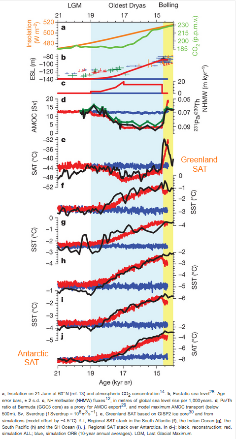
From He et al 2013
Figure 2
We can see that orbital forcing on its own has just about no impact on any of the main temperature metrics, and we can see that Antarctica and Greenland have different temperature histories in this period.
- We can see that their ALL model did a reasonable job of reconstructing the main temperature trends.
- We can also see that it did a poor job of capturing the temperature fluctuations on the scale of centuries to 1kyr when they occurred.
For reference here is the Greenland record from NGRIP from 20k – 10kyrs BP:
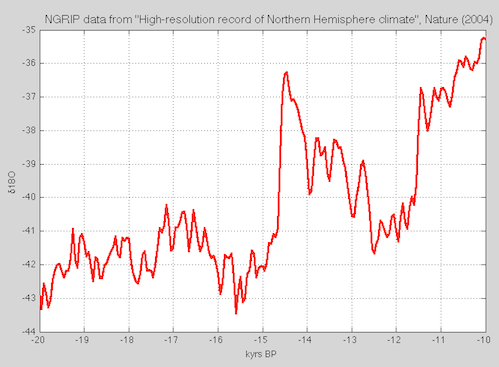
Figure 3 – NGRIP data
We can see that the main warming in Greenland (at least this location in N. Greenland) took place around 15 kyrs ago, whereas Antarctica (compare figure 1 from Shakun et al) started its significant warming around 18 kyrs ago.
The paper basically demonstrates that they can capture two main temperature trends due to two separate effects:
- The “cooling” in Greenland from 19k-17k years with a warming in Antarctica over the same period – due to the MOC
- The continued warming from 17k-15k in both regions due to GHGs
Note that my NGRIP data shows a different temperature trend from their GISP data and I don’t know why.
Let’s understand what the model shows – this data is from their Supplementary data found on the Nature website.
First, 19-17 kyrs ago, Antartica (AN) has a significant warming, while Greenland (GI) has a bigger cooling:
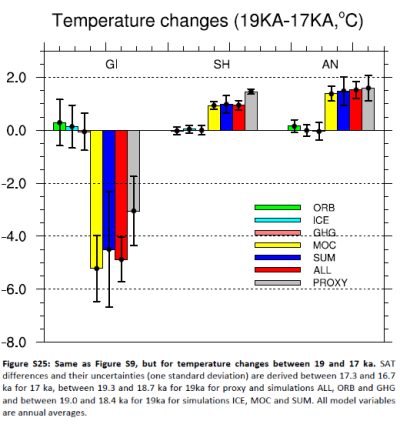
Figure 4
Note that the MOC (yellow) is the simulation that produces both the GI and AN change. (SUM is the values of the individual runs added together, while ALL is the simulation with all forcings combined).
Second, 17 – 15 kyrs ago, Antartica (AN) continues its warming and Greenland (GI) also warms:
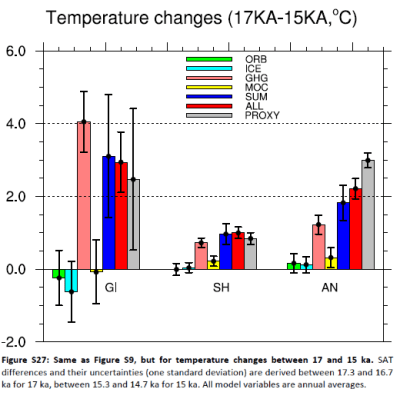
Figure 5
Note that GHG (pink) is the primary cause of the temperature rises now.
We can see the temperature trends over time as a better way of viewing it. I added some annotations because the layout wasn’t immediately obvious (to me):
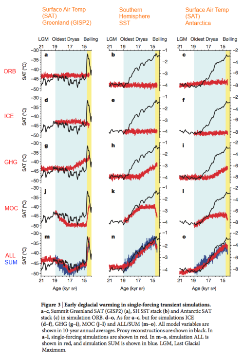
Figure 6 – Red/blue annotations on side, and orange annotations on top
Again, as with figure 1, we can see that the main trends are quite well simulated but the model doesn’t pick shorter period variations.
The MOC in brief
A quick explanation – the MOC brings warmer surface tropical water to the high northern latitudes, warming up the high latitudes. The cold water returns at depth, making a really big circulation. When this circulation is disrupted Antarctica gets more tropical water and warms up (Antarctica has a similar large scale circulation running from the tropics on the surface and back at depth), while the northern polar region cools down.
It’s called the bipolar seesaw.
When your pour an extremely big vat of fresh water into the high latitudes it slows down, or turns off, the MOC. This is because fresh water is not as heavy as salty water, it can’t sink and it slows down the circulation.
So – if you have lots of ice melting in the high northern latitudes it flows into the ocean, slowing down the MOC, cooling the high northern latitudes and warming up Antarctica.
That’s what their model shows.
The available data on the MOC supports the idea, here is the part d from their fig 1 – the black line is the proxy reconstruction:
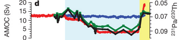
Figure 7
The units on the left are volume rates of water flowing between the tropics and high northern latitudes.
What Did Orbital Forcing do in their Model?
If we look back at their figure 1 (our figure 2) we see no change to anything as a result of simulation ORB so the abstract might seem a little confusing when their paper indicates that insolation, aka the Milankovitch theory, is what causes the whole chain of events.
In their figure 2 they show a geographical look of polar and high latitude summer temperature changes as a result of simulation ORB.
The initial increase of the mid-latitude to high-latitude NH spring–summer insolation between 22 and 19 kyr BP was about threefold that in the SH (Fig. 2a, b). Furthermore, the decrease in surface albedo from the melting of terrestrial snow cover in the NH results in additional net solar flux absorption in the NH (Supplementary Figs 12–15). Consequently, NH summers in simulation ORB warm by up to 2°C in the Arctic and by up to 4°C over Eurasia, with an area average of 0.9°C warming in mid to high latitudes in the NH (Fig. 2c, e).
In their model this doesn’t affect Greenland (for reasons I don’t understand). They claim:
Our ORB simulation thus supports the Milankovitch theory in showing that substantial summer warming occurs in the NH at the end of the Last Glacial Maximum as a result of the larger increase in high-latitude spring–summer insolation in the NH and greater sensitivity of the land-dominated northern high latitudes to insolation forcing from the snow–albedo feedback.
This orbitally induced warming probably initiated the retreat of NH ice sheets and helped sustain their retreat during the Oldest Dryas.
[Emphasis added].
Analysis
1. If we run the same orbital simulation at 104, 83 or 67 kyrs BP (or quite a few other times) what would we find? Here are the changes in insolation at 60°N from 130 kyrs BP to the present:
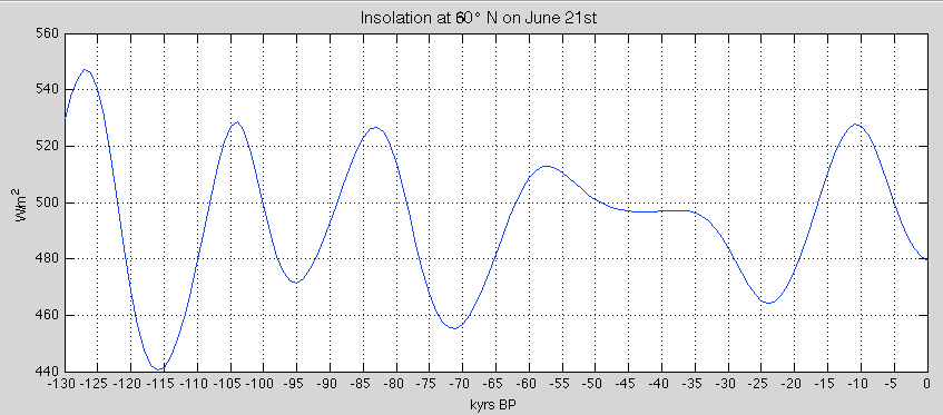
Figure 8
It’s not at all clear what is special about 21-18 kyr BP insolation. It’s no surprise that a GCM produces a local temperature increase when local insolation rises.
2. The meltwater pulse injected in the model is not derived from a calculation of any ice melt as a result of increased summer temperatures over ice sheets, it is an applied forcing. Given that the ice melt slows down the MOC and therefore acts to reduce the high latitude temperature, the MOC should act as a negative feedback on any ice/snow melt.
4. The Smith & Gregory 2012 paper that we look at in Part Nine maybe has different effects from the individual forcings to those found by He et al. Because 20 – 15 kyrs is a little compressed in Smith & Gregory I can’t be sure. Take, for example, the effect on (only) ice sheets during this period. Quite an effect in SG2012 over Greenland, nothing in He et al (see fig 6 above).

From Smith & Gregory 2012
Figure 9
Conclusion
It’s an interesting paper, showing that changes in the large scale ocean currents between tropics and poles (the MOC) can account for a Greenland cooling and an Antarctic warming roughly in line with the proxy records. Most lines of evidence suggest that large-scale ice melt is the factor that disrupts the MOC.
Perhaps high latitude insolation changes at about 20 kyrs BP caused massive ice melt, which slowed the MOC, which warmed Antarctica, which led (by mechanisms unknown) to large increases in CO2, which created positive feedback on the temperature rise and terminated the last ice age.
Perhaps CO2 increased at the same time as Antarctic temperature (see the brief section on Parrenin et al 2013 in Part Eleven), therefore raising questions about where the cause and effect lies.
To make sense of climate we need to understand why:
a) previous higher insolation in the high latitudes didn’t set off the same chain of events
b) previous temperature changes in Antarctica didn’t set off the same chain of events
c) whether the temperature changes produced in simulation ORB can account for enough ice melt seen in the MOC changes (and what feedback effect that has)
And of course, we need to understand why CO2 increased so sharply at the end of the last ice age.
Articles in the Series
Part One – An introduction
Part Two – Lorenz – one point of view from the exceptional E.N. Lorenz
Part Three – Hays, Imbrie & Shackleton – how everyone got onto the Milankovitch theory
Part Four – Understanding Orbits, Seasons and Stuff – how the wobbles and movements of the earth’s orbit affect incoming solar radiation
Part Five – Obliquity & Precession Changes – and in a bit more detail
Part Six – “Hypotheses Abound” – lots of different theories that confusingly go by the same name
Part Seven – GCM I – early work with climate models to try and get “perennial snow cover” at high latitudes to start an ice age around 116,000 years ago
Part Seven and a Half – Mindmap – my mind map at that time, with many of the papers I have been reviewing and categorizing plus key extracts from those papers
Part Eight – GCM II – more recent work from the “noughties” – GCM results plus EMIC (earth models of intermediate complexity) again trying to produce perennial snow cover
Part Nine – GCM III – very recent work from 2012, a full GCM, with reduced spatial resolution and speeding up external forcings by a factors of 10, modeling the last 120 kyrs
Part Ten – GCM IV – very recent work from 2012, a high resolution GCM called CCSM4, producing glacial inception at 115 kyrs
Pop Quiz: End of An Ice Age – a chance for people to test their ideas about whether solar insolation is the factor that ended the last ice age
Eleven – End of the Last Ice age – latest data showing relationship between Southern Hemisphere temperatures, global temperatures and CO2
Thirteen – Terminator II – looking at the date of Termination II, the end of the penultimate ice age – and implications for the cause of Termination II
Fourteen – Concepts & HD Data – getting a conceptual feel for the impacts of obliquity and precession, and some ice age datasets in high resolution
Fifteen – Roe vs Huybers – reviewing In Defence of Milankovitch, by Gerard Roe
Sixteen – Roe vs Huybers II – remapping a deep ocean core dataset and updating the previous article
Seventeen – Proxies under Water I – explaining the isotopic proxies and what they actually measure
Eighteen – “Probably Nonlinearity” of Unknown Origin – what is believed and what is put forward as evidence for the theory that ice age terminations were caused by orbital changes
Nineteen – Ice Sheet Models I – looking at the state of ice sheet models
References
Northern Hemisphere forcing of Southern Hemisphere climate during the last deglaciation, He, Shakun, Clark, Carlson, Liu, Otto-Bliesner & Kutzbach, Nature (2013) – free paper (there is considerable supplementary information probably only available on the Nature website)


On point b) in the conclusion, many people don’t appreciate how much variation occurred during the last glacial.
Here is a figure from Timing of Millennial-Scale Climate Change in Antarctica and Greenland During the Last Glacial Period, Thomas Blunier and Edward J. Brook, Science (2001):
So if the temperature change that occurred in Antarctica between 19 – 17 kyr initiated a chain of events to cause the termination – why didn’t the many larger ones in the previous 70 kyrs terminate the ice age then ?
Another way of looking at point b) is from Glacial terminations as southern warmings without northern control, W. Wolff, H. Fischer & R. Röthlisberger, Nature (2009):
This figure compares three Antarctic warming events during the last glacial with three actual ice age terminations. You can see that the first 2,000 years are similar enough in terms of magnitude and rate of change that there is nothing unusual about the start of these three terminations.
The paper comments on this particular point:
This paper, by the way, was one of the many that got a quick review in Part Six – “Hypotheses Abound”.
thanks, for the standard expolanation of bipolar seesaw. There’s still some things that make me question it’s certainty, but I cannot put my finger on it. Offering instead a very doubtful mechanism for that. Could it be the difference of animal vs. plant dispersion speeds that have lead to this, resource (plant matter) depletion in high northern/southern latitudes by the more mobile animals? This would tie it nicely to the Arctic exploration currently happening, but likely there’s no evidence of this. The fact that the warming seems to happen first in the SH leads to a question, when did Australia become a desert? Is there a ‘green Sahara’ type of thing also here?
So why not pay attention to small scale changes in the MOC, particularly the AMOC? It’s fairly obvious to anyone who looks at the data without an axe to grind that it wasn’t a combination of a change in TSI and aerosols that caused the rapid increase in warming during the early part of the twentieth century and the slowdown in warming in the middle.
But then you would have to pay attention to the fact that Antarctic sea ice has been increasing at a rate about half as fast as Arctic sea ice is decreasing rather than sweeping it under the rug by claiming that the the Antarctic circumpolar vortex and accompanying circumpolar ocean current somehow isolates it from the rest of the planet. You also wouldn’t be able to attribute almost all of the recent warming to ghg’s and the average model climate sensitivity would then even further above the real sensitivity than it appears to be now.
DeWitt,
Do you have the timeseries of both Greenland and Antarctica over the last 110 years or so?
I’m getting together the various timeseries from NGRIP & EPICA. It would be interesting to see what similarities there are between the last glacial period, the pre-industrial Holocene and the last century..
One-to-one coupling of glacial climate variability in Greenland and Antarctica, EPICA Community Members, Nature (2006) is a good paper to see the past relationships, along with Wolff et al (2009), cited above.
I also just downloaded the MOC data from the RAPID program, which is a new program in place for the last 8+ years.
There’s a lot of variation in the MOC:
SoD,
What I’ve been looking at is the AMO index which covers the last 150 years or so starting in 1856. It’s a monthly statistic. You won’t see the variation of interest, which has a period of ~65 years, in an 8 year plot, especially since the AMO index is currently at the cyclical peak. The big question is whether the cycle will repeat again. We won’t know the answer to that for at least another ten years.
I should look at the correlation of the Arctic sea ice anomaly or the rate of change of the anomaly and the RAPID MOC data.
SoD – thanks for this continued discussion. I think your “a” and “b” points and the various lines of evidence you’ve posted do appear to me to be suggesting that the MOC see-saw event (random timing?) needs to coincide with some portion of the orbital forcing curve for a deglaciation. If the MOC timing is wrong, no deglaciation. If the orbital forcing peak happens without an MOC see-saw, no deglaciation. Plausible?
Arthur,
You say “..needs to coincide with some portion of the orbital forcing curve for a deglaciation..” but I don’t understand why, or if I have implied that?
I reread Wolff et al 2009 for what must be the 5th time just now – hope I finally get all their points – in brief, the ice age termination happens because an Antarctic warming did not get halted by a Greenland warming (aka “DO event”). Something prevented it. They say that this could be due to orbital effects but don’t really come up with any.
So, if you like, I will paraphrase their theory, with apologies to Eric Wolff and his colleagues if I have it all wrong:
It’s a theory, and the evidence seems to be there:
– Certainly Southern warming leads Northern warming in a large number of “in-glacial warmings” (but see note).
– Certainly lots of Southern warming took place without a termination.
The “deterministic mechanism” for one part is not identified.
If only we can just find a changing insolation curve to pin it all on..
Note – Synchronicity of Antarctic temperatures and local solar insolation on orbital timescales, Thomas Laepple, Martin Werner & Gerrit Lohmann, Nature (2011):
[Emphasis added]
Louise Sime & (the now locally famous) Eric Wolff replied in Nature that year, and Laepple et al respond to their criticisms, including:
More on this later (when I can understand it).
The lead author of the paper, Feng He, was kind enough to respond to a few of my questions:
1. Did you run the same ORB simulation at earlier times of higher insolation in the NH high latitudes – e.g. 104, 83 or 67 kyrs?
Given the smaller ice sheets and lower GHGs surely the effects would be greater than those simulated at 20 kyrs?
2. Fig 1e (Greenland) with simulation ORB shows a flat line. But the text and figs 2 indicate significant high latitude NH summer warming (ORB model).
I can see that from 22-19kyrs the other seasons balance out the summer warming but before 15kyrs the average temperature from all seasons is clearly positive (in fig 2d).
Also the legend for Fig 1e says “model offset by -4.5’C” – I just wanted to check I understand this correctly, the model line should be moved down by 4.5’C and the difference between ALL and proxy at 17kyrs would be around 5’C (i.e., ALL cooler than proxy by 5’C at 17kyrs?).
See note 1 below.
3. Was any calculation made of the ice sheet melt from the high latitude NH summer warming and autumn cooling? The text says: “This orbitally induced warming probably initiated the retreat of NH ice sheets” but I couldn’t find any link to the MOC changes that the model indicates really got the termination moving along.
See note 2 below.
Note 1 –
There is a general problem in ice age modeling due to model resolution – basically the GCM has each “cell” or “grid” at the same altitude, but there are lots of smaller high altitude regions that are colder. One paper that looked at this problem from the point of the last glacial inception 115kyrs BP showed that increasing the resolution helped create perennial snow cover (we looked at this problem in earlier articles in this series).
The role of GCM resolution in simulating glacial inception, Steve Vavrus, Gwenaëlle Philippon-Berthier, John E. Kutzbach and William F. Ruddiman, The Holocene (2011)
It’s an interesting paper, but also generates more questions than answers for me. Like, what happens when we increase the resolution by a factor of 10? Models attempting perennial snow cover got the right answer with very simple models, then the “wrong answer” with better models, then the right answer with even better models.. It’s all fine if you already know what the correct answer is..
Note 2 –
I believe this paper is Collapse and rapid resumption of Atlantic meridional circulation linked to deglacial climate changes, J. F. McManus, R. Francois, J.-M. Gherardi, L. D. Keigwin & S. Brown-Leger, Nature (2004)
In The Confirmation Bias – Or Why None of Us are Really Skeptics I commented on The Black Swan by Nassim Nicholas Taleb on the confirmation bias.
In brief, to test a theory you should be looking for evidence that would disprove the theory but most of us look for evidence to bolster our theory.
I wonder if anyone at all has invested GCM time (I know it’s a precious resource) into “falsifying” the orbital hypothesis as far as the last glacial termination is concerned, by running the same simulation over say 90 – 80 kyrs BP.
My impression is that all this research is presently in the phase where the question is:
– Can we make our model reproduce the known history at some level of accuracy?
rather than
– Does the present understanding of the Earth system uniquely predict the main features of the glacial cycles?
We can be fairly satisfied with the level of understanding when we can answer the second question positively. Answering the first question positively is better than answering it negatively, but the second question is the more important one.
Pekka,
That might be the case.
An alternative point of view is that current research is attempting to generate the necessary basic understanding of the climate system, and models are an essential part of that.
Without a model we can’t test the idea properly. Finding which models reproduce history and which ones don’t allows much improvement of basic understanding of how climate works. (I realize you accept these last 2 sentences, many people read this blog who don’t appreciate the necessity/benefit of models).
In the more politically-charged areas of “climate debate”, of course, it might seem as you describe. In a couple of hundred papers on ice ages it seems more like my “alternative point of view” above.
SoD,
This recent discussion of ice ages seems to have a different nature than most of your earlier posts.
The earlier posts have discussed mainly issues where science has produced a basic agreement shared by most, often all, climate scientists. The details may be more uncertain but those uncertainties have not been the main point of the posts.
Now you have entered a field where “hypotheses abound”, and both the posts and the ensuing discussion are on issues where the active scientists seem to be almost as uncertain as we are in discussing these theories. (It would not be surprising if some of us would feel more certain based on the power of ignorance.)
SoD,
I agree.
However, current models are being misused when it’s claimed that they can describe details of the future climate Articles like this:
Increasing Frequency of Extreme El Niño Events due to Greenhouse Warming are closer to science fiction than science.
I checked for curiosity the availability of insolation data and found the Lasker et al 2004 integration and the precompiled Fortran program INSOLA from
http://www.imcce.fr/Equipes/ASD/insola/earth/earth.html
I checked the results for 60N for the latest 130 kyr. The result is similar enough to what you present for all the conclusions made here, but not identical. The most visible difference is a clear minimum around -46 kyr. Insolation at that minimum is 494 and at the following maximum at -37 kyr is 500. Your curve is essentially flat in that region without a significant minimum. There are observable differences also in the other maximum and minimum values.
I have no idea about the reason for these differences.
I have converted INSOLA to C++ as I’m presently more comfortable with C and C++ and have better tools for those.
[…] 2014/01/16: TSoD: Ghosts of Climates Past – Twelve – GCM V – Ice Age Termination […]
[…] Twelve – GCM V – Ice Age Termination – very recent work from He et al 2013, using a high resolution GCM (CCSM3) to analyze the end of the last ice age and the complex link between Antarctic and Greenland […]