In Part Four we started looking at the changes in solar insolation due to the different orbital effects.
Eccentricity itself has a negligible effect on solar insolation. Obliquity and precession change the (geographic and temporal) distribution of solar radiation, but not the annual amount.
Here is the annual variation for each season at 65ºN:
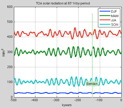
Figure 1
There is less variation by year than the value on any given day (compare fig 5 & 6) in Part Four.
Here is the corresponding graph for 55ºN:
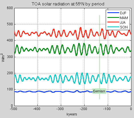
Figure 2
Of course, higher solar radiation in one part of the year due to tilt, or obliquity, means less solar radiation in the “opposite” part of the year.
In the graphs above we see that at the peak of the Eemian inter-glacial, JJA (June-July-August) radiation is a minimum, MAM (March-April-May) is on the upswing towards its peak, SON is on a downswing past its peak and of course, DJF is very low and not changing much because there isn’t much sun at high latitudes during the winter.
So what about the annual variation? Let’s zoom in on the period around the Eemian inter-glacial. The top graph shows the daily average insolation for four different years, and the bottom graph shows the annual average by year:
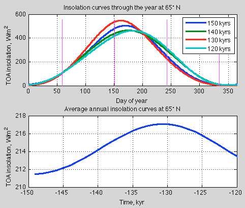
Figure 3
And for reference the annual variation over the last 500 kyrs:
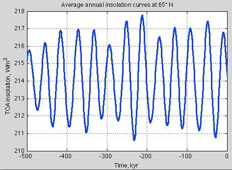
Figure 4
And the same data for 55ºN:
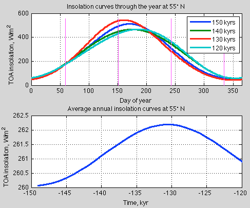
Figure 5
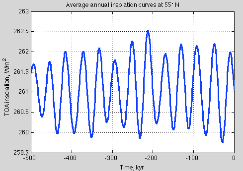
Figure 6
As we would expect, the peaks and troughs occur at the same times for 55ºN and 65ºN.
What is different between the two latitudes is the change in annual insolation with time at a given latitude. The 65ºN insolation varies by 7 W/m² over the last 500 kyrs, while the 55ºN figure is not quite 3 W/m². By comparison 45ºN varies by less than 1 W/m².
Around the 30 kyrs centered on the Eemian inter-glacial, the variation is:
- 65ºN – 5.5 W/m²
- 55ºN – 2.2 W/m²
- 45ºN – 0.3 W/m²
And if we take the steepest part of the increase from 145 kyr – 135 kyr, we get a per century value of:
- 65ºN – 40 mW/m² per century
- 55ºN – 25 mW/m² per century
- 45ºN – 2 mW/m² per century
- (and in the southern hemisphere there were similar reductions in insolation over this period)
Now by comparison, due to increases in atmospheric CO2 and other “greenhouse” gases, the “radiative forcing” prior to any feedbacks (i.e., all other things remaining the same) is about 1.7 W/m² over 130 years, or 1.3 W/m² per century.
Now this has been applied globally of course, but in any case recent changes have been 30 – 50 times the rate of increase of high latitude radiative change during one of the key transitions in our past climate.
These values and comparisons aren’t aimed at promoting or attacking any theory, they are just intended to get some understanding of the values in question.
Of course, annual changes are smaller than seasonal changes. So let’s look back at the seasonal values around 120 kyrs – 150 kyrs:
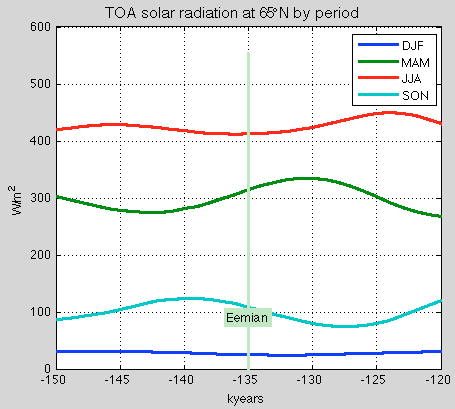
Figure 7
And let’s make it easier to understand the changes by looking at the anomaly plot (signal minus the mean for each season):
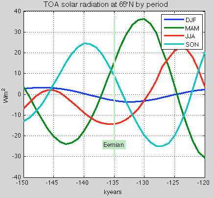
Figure 8
We have quite large changes (comparatively) in each season. For example, the March-April-May figure increases by 60 W/m² from 143 kyrs ago to 130 kyrs ago, which is almost 0.5 W/m² per century, on a par with recent radiative forcing changes due to GHGs.
The problem with just looking at MAM – and is the reason why I started plotting all these results – is if the increase in MAM insolation caused more rapid ice melt at the end of winter, then didn’t the similarly large reduction in SON (autumn) insolation cause more ice to be there ready for spring? Each year has all the seasons so the whole year has to be considered..
And if there is such a clear argument for one season being some kind of dominant force compared with another season (some strong non-linearity), why isn’t there a consensus on what it is (along with some evidence)?
Huybers & Wunsch (2005) noted:
Taking these two [Milankovitch and chaos] perspectives together, there are currently more than 30 different models of the seven late Pleistocene glacial cycles.
Lastly, for interest, here is a typical spectral power plot of the TOA solar insolation (normalized). This one happens to have each season as a separate curve, but there isn’t much difference between each period so the plots pretty much overlay each other. The 3 vertical magenta lines represent (from left to right) the frequencies of 41 kyrs, 23 kyrs and 19 kyrs:
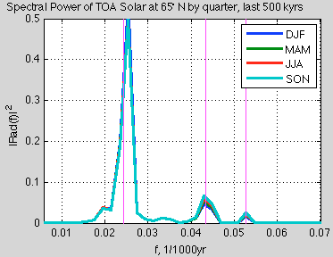
Figure 7
In some later articles we will look at the spectral characteristics of the ice age record so knowing the spectral characteristics of orbital effects on insolation is important.
Articles in the Series
Part One – An introduction
Part Two – Lorenz – one point of view from the exceptional E.N. Lorenz
Part Three – Hays, Imbrie & Shackleton – how everyone got onto the Milankovitch theory
Part Four – Understanding Orbits, Seasons and Stuff – how the wobbles and movements of the earth’s orbit affect incoming solar radiation
Part Six – “Hypotheses Abound” – lots of different theories that confusingly go by the same name
Part Seven – GCM I – early work with climate models to try and get “perennial snow cover” at high latitudes to start an ice age around 116,000 years ago
Part Seven and a Half – Mindmap – my mind map at that time, with many of the papers I have been reviewing and categorizing plus key extracts from those papers
Part Eight – GCM II – more recent work from the “noughties” – GCM results plus EMIC (earth models of intermediate complexity) again trying to produce perennial snow cover
Part Nine – GCM III – very recent work from 2012, a full GCM, with reduced spatial resolution and speeding up external forcings by a factors of 10, modeling the last 120 kyrs
Part Ten – GCM IV – very recent work from 2012, a high resolution GCM called CCSM4, producing glacial inception at 115 kyrs
Pop Quiz: End of An Ice Age – a chance for people to test their ideas about whether solar insolation is the factor that ended the last ice age
Eleven – End of the Last Ice age – latest data showing relationship between Southern Hemisphere temperatures, global temperatures and CO2
Twelve – GCM V – Ice Age Termination – very recent work from He et al 2013, using a high resolution GCM (CCSM3) to analyze the end of the last ice age and the complex link between Antarctic and Greenland
Thirteen – Terminator II – looking at the date of Termination II, the end of the penultimate ice age – and implications for the cause of Termination II
References
Obliquity pacing of the late Pleistocene glacial terminations, Peter Huybers & Carl Wunsch, Nature (2005)
All graphs produced thanks to the Matlab code supplied by Jonathan Levine.


SoD, there are green lines marked with Eemian at -135kyrs.
But this is approximately the start of the warming, still deep in the glacial. The Eemian was rather from -130kyrs to -120 kyrs, I think.
Uli,
Dating these events has some uncertainty.
Broecker’s 1992 Nature paper – Upset for Milankovitch Theory – noted that, based on 234U-230Th dates from Devil’s Hole in Nevada, the previous inter-glacial termination began at 145,000 years. This contrasts with earlier dates given of around 128,000 years.
I will be digging deeper into the dating of ice ages in future articles because it is a big subject, and much of the explicit dating methodology (and probably now dating bias) was tied to Milankovitch cycles.
I’m currently reading a lot of papers from the EPICA project, mostly from 2008 onwards.
SOD: I’m not sure what the word “termination” really means when applied to an ice age. It could be the first DATE at which ice volume began to markedly decrease or it could be the PERIOD of most rapid melting (constant steepest slope). These changes in ice volume presumably lag behind changes in temperature, and we measure both by a variety of proxies. Recent history includes the Last Glacial Maximum, “termination”, and the Holocene, with the possibility that there are periods between or that aren’t given names or possibly periods of overlap.
The Holocene officially began 11,700 years BP, which is well before the end of the period of rapid sea level rise ended about 8,000 ybp. Wikipedia says the LGM was between 26,500 and 19,000–20,000. A brief search didn’t uncover a date or range of dates for “termination” or a definition.
SoD, 145kyrs seems outside the estimates I know.
Do not miss this EPICA paper about the EDC3 chronology:
http://www.clim-past.net/3/485/2007/cp-3-485-2007.html
[…] « Ghosts of Climates Past – Part Five – Obliquity & Precession Changes […]
[…] impact of an increase of 50W/m² (over 10,000 years) in summer at 65ºN – see figure 1 in Ghosts of Climates Past – Part Five – Obliquity & Precession Changes. What effect does the simultaneous spring reduction at 65ºN have. Do these two effects cancel […]
[…] Part Five – Obliquity & Precession Changes – and in a bit more detail […]
This article suggests that precession and albedo are responsible for Interglacial warming. In which case, the sequence of events that are required to produce an interglacial period become:
a. Interglacials are initiated by precessional Milankovitch cycles.
b. Regional insolation increase in the NH is the primary forcing.
c. Milankovitch forcing is enhanced by albedo feedbacks, not CO2.
d. For insolation to have an effect on ice sheets, their albedo must be lowered.
e. This is achieved via the dust-storms that precede every Interglacial.
f. The dust-storms are caused by CO2 reaching critically low levels.
g. The lack of CO2 causes global plant die-back and barren lands.
h. Dust from these barren lands is blown across the ice for 10,000 years.
i. And now we have all the elements in place to produce an Interglacial.
Albedo regulation of Ice Ages, with no CO2 feedbacks
https://www.academia.edu/16866736/Albedo_regulation_of_Ice_Ages_with_no_CO2_feedbacks
Sincerely,
Ralph Ellis
You need to read the complete series. The evidence that precessional Milankovitch cycles have initiated the recent interglacials is actually quite weak. It’s also probably not necessary to invoke CO2 for a reduction in plant cover. A decrease in global precipitation caused by lower specific humidity at the lower global temperature is probably sufficient to explain desertification leading to higher atmospheric dust levels.