In previous articles we have discussed the Milankovitch hypothesis – classically paraphrased as:
Solar insolation at 65ºN in summer determines the start and end of ice ages – with minimum summer insolation preventing snow melt at high latitudes which allows perennial snow cover, positive feedback from reflected solar radiation and the consequent growth of ice sheets.
Conversely maximum solar insolation at high latitudes causes ice sheets to melt and (with the same positive feedback effect) ends the ice age.
And “summer” is usually taken as the insolation on June 21st even if it is a somewhat arbitrary date (we can also average over a month or the season).
So I produced a few contour plots, showing the insolation anomaly by latitude and day of year compared with the present for 8 different years between the start of the last ice age (about 115 kyrs ago) and today.
The challenge for readers is to identify which graph corresponds to the end of the last ice age. And some kind of reason why you chose that graph.
I made them a little smaller so that they could be more easily compared – just click on each set to expand.
The x-axis (left to right) is day of year, and June 21st is about day 200 (actually it is 172, thanks to Climateer for pointing this out!). The y-axis (bottom to top) is the latitude. The colors represent the same in each graph and the contour lines are 10 W/m² apart.
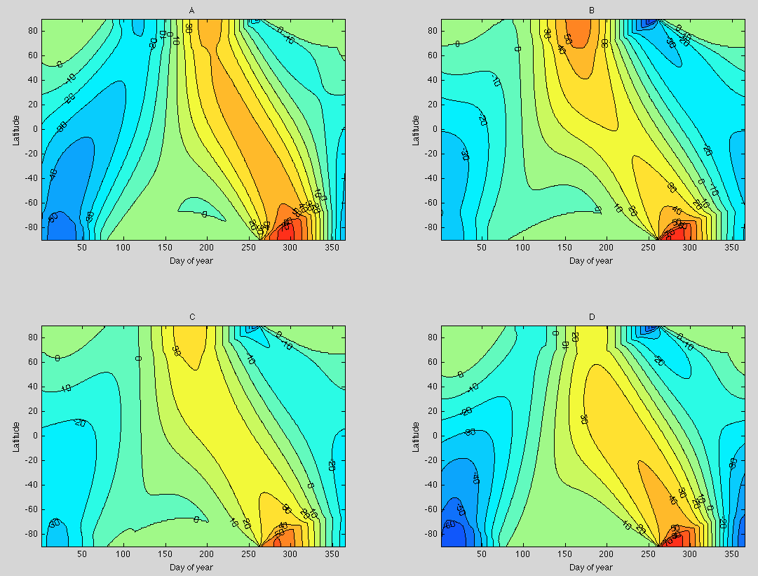
Figures A – D – Click for larger view

Figures E – H – Click for larger view
Articles in the Series
Part One – An introduction
Part Two – Lorenz – one point of view from the exceptional E.N. Lorenz
Part Three – Hays, Imbrie & Shackleton – how everyone got onto the Milankovitch theory
Part Four – Understanding Orbits, Seasons and Stuff – how the wobbles and movements of the earth’s orbit affect incoming solar radiation
Part Five – Obliquity & Precession Changes – and in a bit more detail
Part Six – “Hypotheses Abound” – lots of different theories that confusingly go by the same name
Part Seven – GCM I – early work with climate models to try and get “perennial snow cover” at high latitudes to start an ice age around 116,000 years ago
Part Seven and a Half – Mindmap – my mind map at that time, with many of the papers I have been reviewing and categorizing plus key extracts from those papers
Part Eight – GCM II – more recent work from the “noughties” – GCM results plus EMIC (earth models of intermediate complexity) again trying to produce perennial snow cover
Part Nine – GCM III – very recent work from 2012, a full GCM, with reduced spatial resolution and speeding up external forcings by a factors of 10, modeling the last 120 kyrs
Part Ten – GCM IV – very recent work from 2012, a high resolution GCM called CCSM4, producing glacial inception at 115 kyrs
Eleven – End of the Last Ice age – latest data showing relationship between Southern Hemisphere temperatures, global temperatures and CO2
Twelve – GCM V – Ice Age Termination – very recent work from He et al 2013, using a high resolution GCM (CCSM3) to analyze the end of the last ice age and the complex link between Antarctic and Greenland
Thirteen – Terminator II – looking at the date of Termination II, the end of the penultimate ice age – and implications for the cause of Termination II
Fourteen – Concepts & HD Data – getting a conceptual feel for the impacts of obliquity and precession, and some ice age datasets in high resolution
Fifteen – Roe vs Huybers – reviewing In Defence of Milankovitch, by Gerard Roe
Sixteen – Roe vs Huybers II – remapping a deep ocean core dataset and updating the previous article
Seventeen – Proxies under Water I – explaining the isotopic proxies and what they actually measure
Eighteen – “Probably Nonlinearity” of Unknown Origin – what is believed and what is put forward as evidence for the theory that ice age terminations were caused by orbital changes
Nineteen – Ice Sheet Models I – looking at the state of ice sheet models


Assuming the figures are tagged , “B” appears most consistent with the trigger for ceasing glacial demanded by the Milankovitch hypothesis. High insolation at +-80 latitude straddles the 200 day vertical, although is not precisely on it.
Oops LaTeX did not work: I wanted “A&B\\C&D”.
June 21 = Julian Day 172
I kinda cheated, so I’ll refrain, but thought provoking quiz.
Climateer,
thanks, you are correct, I updated the text.
I also think its B because the insolation at 65 degrees north in summer is the highest. Its so obvious though that I think it must be a trick question 🙂 Of course it’s also assuming the Milancovitch hypothesis is correct.
As we are comparing with the present, not with a mean value, the first question is how the present deviates from the average – or alternatively we can try to find out, how the time from the end of last ice age compares with the periods of the contributing factors. Many of the alternatives do not fit this case at all, two or three look more promising, but I leave for now open, what those alternatives and my first guess are.
Pekka,
When you say “the periods of the contributing factors” do you mean the change over a given period?
For each of the above times I can produce the change over the last 5 kyrs or 10 kyrs or whatever time difference you want.
SoD,
I meant the various periodic phenomena in the orbital parameters that affect insolation, and considering how much the influence the difference between today and the end of last ice age.
I didn’t want to tell more.
One intriguing feature in the graphs is how the strongest deviation is typically at South pole in the beginning of the year, moves through all latitudes to the North pole during the first part of the year. After a while a different deviation has formed in the North and moves in the opposite direction reaching the South pole before the end of the year.
I have been wondering, what that tells about the present situation relative to the mean values of insolation at various times during the year.
And now, we reveal the dates corresponding to each of the graphs in the article:
These are 100 kyrs BP, 10 kyrs BP, 55 kyrs BP and 79 kyrs BP. The first, third and fourth all took place long before the ice age ended. The second graph, 10 kyrs ago, was 8kyrs into the current interglacial.
These are 50 kyrs BP, 30 kyrs BP, 18 kyrs BP and 68 kyrs BP.
The correct answer, highlighted, is G = 18 kyrs ago.
No prizes can be awarded but hopefully it’s clear that predicting the end of an ice age from insolation curves is quite difficult.
Here is the June 21st 65’N insolation curve plotted against time:
Kudos.
Frank,
In an earlier comment in one of these threads I listed several phases, This time I decided to pick just two and consider even the interglacial as a turning point between those two.
The word chaos has come up a couple of time recently. I don’t think that it’s really relevant here. The basic sawtooth does not look at all like chaos, neither does that part of variability that’s very likely forced by changes in insolation. The main effects have rather a deterministic appearance while the chaotic variation occurs on a smaller scale. We may very well have “attractors” and transitions between those on a deterministic basis, and that’s what I image to see in the full glacial cycles.
I linked the above reply to a wrong comment. It should be linked to that of Frank below.
The obvious question is whether the insolation for some other time period (all summer months?) or latitude. WIth 3-4 km thick ice sheets at the LGM (about 20 degC colder at the top than at ground level), ice sheets probably melt from the sides, not the top. That is likely to start far south of 65 degN, the latitude where ice sheet initiation starts.
Does anyone know how much the ice sheets depressed the ground at the LGM. The center of Greenland today is below sea level. I was surprised to read somewhere that the outline of the Antarctic continent on maps today shows where land would meet the ocean after ice sheet melting and glacial isostatic rebound. The amount of land above sea level today is smaller than shown on the map. (I hope I got this right.) Perhaps glacial terminations are initiated when compressed continents allow the ocean to attack the base of the ice sheet below sea level. Tides might drive ocean water into and out of the base of the ice sheet.
Frank
You can see some area-averaged insolation values as Hovmoller plots in comments on Part Eleven and subsequent.
You can “mentally average” over a seasonal period because the plot is time in years on the x-axis and days of the year on the y-axis. If you think one time region is the key I’m sure I can produce an appropriate plot.
But also, take a look at the comments on Part Twelve where I show the Antarctic warmings that take place prior to the NH warmings (not necessarily obvious in those plots but the lead is clear via synchronizing from CH4 records in both polar cores).
The SH leads the termination. Why then, is NH insolation a key?
There were lots of SH warmings that preceded NH warmings. Why did the specific one produce a termination?
What caused all the SH warmings?
Lots of questions.
SOD: The Hovmoller plots suggest that the lack of radiation in the summer months was greatest about 110 ka ago, a little before the 115 ka date for initiation mentioned in your posts. Placing more emphasis on spring+summer shifts the period of least irradiation closer to 115 ka, but diminishes the amplitude of the change.
Changes in irradiation at 65 degN might initiate an ice age, but they probably don’t have any effect DURING an ice age. Termination certainly isn’t the inverse of initiation. I would think that terminations begin at 45 or 50 degN at southern edges of the ice sheet where the ice isn’t high enough to be cooled by altitude. Does the relative importance of eccentricity, precession and obliquity change with latitude?
Frank,
Continuing to flog the the deceased equine: IMO, you’re wasting your time trying to understand glacial inception. The current climate has two modes as far as I can tell, glacial and glacial termination. Absent intervention in the form of a massive injection of CO2 into the atmosphere, what we call interglacial climate isn’t stable. It doesn’t need a trigger to begin cooling. If the models don’t show this behavior, it means they are seriously flawed. We also don’t understand glacial termination, which is, again IMO, much more important.
DeWitt: For the most part, I agree with you about the dead horse. The planet may indeed have two stable states: glacial and interglacial. The power needed to form and melt ice sheets is trivial on a global scale (about 0.01 and 0.07 W/m2). However, if our climate varied chaotically between these two states, we wouldn’t see 100,000 and 40,000 year cycles without a periodic mechanism to trigger initiation and termination.
In the case of initiation, SOD suggested that I look at one of the Hovmoller plots he posted to discover an answer to a question about average irradiance over the melting season. I reported what I found, but that dealt only with the conditions near the last initiation (the only initiation on the plot); not what I believed in general.
FWIW, attempts to explain ice ages illustrate for me the ease with which hypotheses in climate science like Milankovitch’s appear to become theories or “accepted science” despite their weaknesses, especially in fundamentals. Fundamental physics says that the change in ice volume – not total ice volume – should vary with power input, yet for decades total ice volume was (and still often is) plotted vs irradiance. I doubt we have learned anything about initiation because of “success” with one of many climate models with a significant Arctic cold bias and with several dozen parameters representing sub-grid processes that can’t be globally optimized. The same skepticism applies to CAGW: overconfidence abounded after 2 decades of relatively rapid warming (1975-1995) even though a fairly similar period of warming (unforced natural variation) was apparent around 1940.
Frank,
What do you think is the time period between the start of Termination II and the start of Termination I ?
And between Termination III and Termination II ?
Frank,
Quasi-periodic oscillations are well known in chaotic systems exhibiting long term persistence. In fact, a switch in period for no apparent reason is exactly what one would expect from such a system. No trigger is required for these systems. Random noise is sufficient.
To me it does not seem to be the case that the Earth has two stable states, but that it has two persistent modes: glaciation and deglaciation. The states of glacial maximum and interglacial seem to be unstable and of very short duration on the geological time scale.
Pekka,
That’s a very interesting way to think about it.
Pekka,
I think that’s what I was trying to say. As usual, your statement is much more elegant than mine.
SOD and DeWItt: I cited 40,000 and 100,000 year cycles based on the spectra analysis of Figure 2 of Part 3. I’ve learned from your posts some dating has been adjusted to align correctly with insolation, but I wasn’t aware that all the regularity in the pattern was due to adjustment. I have been assuming that the record reflected some sort of periodicity or oscillation, rather than chaos, but perhaps I am missing something. How does one distinguish between chaotic and non-chaotic systems? Is ENSO – which is called an oscillation because the period isn’t well-defined – a chaotic system even though it produces a broad peak (0.2-0.5 yr-1?)in the spectral analysis of mean global temperature anomaly? Ice ages appear to be more regular than ENSO. Aside from one large change in frequency about a million years ago, I thought there was reasonable evidence for periodic behavior.
http://en.wikipedia.org/wiki/File:Five_Myr_Climate_Change.svg
Pekka: Looking at the situation your way, aren’t there three states?
1) Ice sheets growing slowly for at least 50,000 years (recently) or 20,000 years (more than 1,000,000 years ago)
2) Ice sheets shrinking (ca 5X faster than they grew).
3) Ice sheets stable and low (interglacials).
There are two ways ice sheets can grow: towards the equator and in altitude.
When ice sheets are big enough, circulation changes due to the land bridge between North America and Asia and a nearly solid land bridge between Asia and Australia/New Guinea. Other changes are caused by the weight of the ice depressing the land underneath (and raising the other areas nearby). I can see why ice albedo feedback keeps ice sheets growing once they start to grow and why circulation or subsidence might eventually stop their growth and begin shrinkage. The mystery to me is why so much ice melts during termination
Regarding Pekka’s “two persistent modes”, I’m sure Pekka doesn’t need me to reply, but my understanding of his insight was that he was speaking of the system as a stochastic one with two statistical modes. My understanding, assuming I understood him correctly, was that transitions were relatively short, so there wasn’t much support for an intermediate state. Continuity, of course, suggests, that the system needs to spend *some* time in-between, even if it is making a transition.
My latest comment higher up should be here. I don’t repeat it here.
In emphasizing the two modes I had in mind the hypothesis that they are so persistent that they are not easily interrupted fully (although there are disturbances during the glaciation). Thus I ponder following questions (to list now only three):
1) What limits the range covered by the glacial cycle? (Perhaps geography and amount of CO2 in circulation).
2) Why are the two modes so persistent?
3) Is the temporal length of the full glacial cycle determined by that range and the natural rates of glaciation and deglaciation rather than Milankovic theory?
Pekka,
Planetary orbits don’t ‘look’ chaotic either. But that doesn’t mean one can calculate backward or forward for billions of years and get the right answer. Statistical tests indicate that the temperature series from ice cores exhibits long term persistence which is a type of chaotic behavior. But in the absence of a complete mathematical description of the system, it can’t be proven. Even in the solar system, the range of the estimate of the magnitude of the Lyupanov coefficient covers more than an order of magnitude. But it does appear to be finite.
The basic issue of chaos is that an arbitrarily small change in initial conditions leads to a finite unpredictable effect given enough time. In the most simple models that have chaos the outcome may have well defined properties like the presence of strange attractors. To have a chaos in that sense it’s essential that the deviation in the initial conditions may be arbitrarily small, no general requirement is given for the ultimate size of the uncertainty in the outcome except that in must exceed some finite limit not depend on the size of the original deviation.
A multi-body problem like orbits of solar system has chaotic behavior, but that’s not important for most issues as precise calculations can be performed over very long periods. That’s an example of the fact that it’s very common that chaos can be discarded in practical analysis.
The atmosphere is definitely chaotic in many ways. That makes long term weather prediction impossible, but that does not necessarily have much effect on many other things. Whether the chaos in the Earth system exhibits anything like strange attractors is totally unknown. It’s not simple chaos like in the simple example of Lorenz, its not understood as chaos in three-body system, it’s spatiotemporal chaos of virtually infinite number of variables.
What we see in the sawtooth of ice ages looks regular, not chaotic. It’s reasonable to search for a deterministic theory that explains that regularity. involving chaos is extremely unlikely to lead anywhere in the understanding of that, because we have no theory of chaos of a system as complex as the Earth system.
Pekka,
You want to see sawtooth type behavior in a system that exhibits long term persistence? Pour sand in a thin stream on a pile. The sand at the peak will build up and collapse. The buildup is slow, the collapse is rapid. So a sawtooth pattern will be imposed on the long term trend of the peak height. The cycle will show periodic behavior, but you won’t be able to predict exactly when the slump will happen. You’ll also get larger slumps at longer intervals. Because the pile gets more unstable as time goes on, the trigger for a slump can be very small. But, of course, that’s the thing we don’t know, why should glacial ice sheets become less stable as they grow larger.
Frank,
Chaotic simply means the system is not deterministic from initial conditions. It doesn’t mean there are no patterns and frequencies.
We don’t have the equations for ENSO. If we did it might be deterministic and have a varying period. Probably ENSO is sensitive to initial conditions and is not deterministic but still has repeatable statistics. (I don’t know much about ENSO).
Chaotic systems with periodic forcing display periodic behavior, but the system will switch between different modes for no apparent reason.
Many choatic systems are very predictable for anything useful we want to know about them.
So chaotic does not necessarily equal unknown, or undefinable, or even “hard to predict”.
First a couple of comments on the broad sweep of history.
Individual contribution of insolation and CO2 to the interglacial climates of the past 800,000 years, Yin & Berger (2012):
And from Eight glacial cycles from an Antarctic
ice core, EPICA (2004):
The evidence presented in Ghosts of Climates Past – Thirteen – Terminator II on the last 2 periods is 123 kyrs and 113 kyrs.
I haven’t dug into the previous deglaciations yet and I don’t know if there is any helpful independent dating that has been done.
But what we do have is a system that has been “consistent” for 8 cycles in a row after switching from a completely different mode.
Or is it 4 cycles in a row of one mode after switching from a completely different mode in the earlier 4 cycles in a row.
And in these last 4 cycles of 100 kyrs, the most recent cycle was 123 kyrs and the one before was 113 kyrs.
What exactly does this all mean? I wonder.
A little more on timings..
Winograd et al 1992, covered in Part Thirteen is cautious on dates for Termination IV and V due to radiometric uncertainties, but given that other dates are uncertain, here is a figure from Duration and Structure of the Past Four Interglaciations, Winograd et al (1997):
This paper is specifically about the duration of interglacials, interesting in its own right, but identifies the termination date graphically.
(From Note 1 in the most recent article, In common ice age convention, the date of a termination is the midpoint of the sea level rise from the last glacial maximum to the peak interglacial condition. This can be confusing for newcomers.)
I identify from the graph:
T-II – 142
T-III – 253
T-IV – 339
T-V – 418
T-VI – 520 (no identifying line for this termination)
This gives us (with TI as 18 kyrs, but perhaps it should be slightly later in time as we are considering the midpoints)
I-II = 124
II-III = 111
III-IV = 86
IV-V = 79
V-VI = 102
The average, no surprise, is 100 kyrs.
Here’s figure 5 from the same paper:
Click for a larger view
Now I’m going to take the time of termination as the time when the proxy measurement really started to increase:
T-II – 154
T-III – 269
T-IV – 354
T-V – 434
T-VI – 522 (taken from figure 2)
The period between the start of terminations:
[corrected, thanks to Arthur Smith]
I-II = 136 (taking the start of TI as about 18kyrs)
II-III = 115
III-IV = 85
IV-V = 80
V-VI = 88
[this following comment is now wrong] The average is 91 kyrs. The last period is clearly the aberration, and the average of the earlier 4 periods is 85 kyrs, which is exactly 4 precessional cycles! Problem solved.
With a small number of irregular periods you can pretty much make up whatever astrology you want..
It will be interesting to see how Dome C (EDC) from Antarctica compares. However, I believe there is some SPECMAP type tuning applied to older records (deeper parts of the core). I am still trying to understand the data.
Yes – G looks totally unremarkable !
I was confused because summer in the N.H. 13,000 years ago was December 21st ! The precession of the earth’s orbital axis is 26,000 years. It may be better to define June 21st as being as mid summer’s day.
Clive,
Our calendar is based on the tropical year, not sidereal year. Thus the NH summer solstice is kept at June 21. I assume that this is true also for the orbital calculations presented by SoD.
From the above curve of SoD we see that 65N insolation was only slightly higher 18 kyears ago. I knew that at a much coarser level. Thus it was obvious that none of the alternatives that indicated large deviations from the present were possible, but I couldn’t decide for sure whether the right one was G or H, but if i remember correctly I considered the cooling parts probably too strong in H.
I haven’t even now figured out, why most of the figures have a very similar shape.
Pekka,
Correct.
The earlier graphs were mostly selected as high or low points of 65’N on June 21st so perhaps we are not seeing a representative sample?
So here are 40k, 35k, 30k, 25k, 20k and 15k vs today:
Click to expand
And also the same vs 10k yrs ago rather than today:

Click to expand
The common feature I see in most of these pictures is that a deviation develops at a pole soon after midsummer and then moves to the other pole reaching that in late spring. There must be a simple reason for that, but so far I haven’t succeeded in building any intuitive picture of that.
I value highly “understanding” the results of calculations well enough to develop such an intuitive picture. That helps greatly in further work related to that subject area.
[…] 2014/01/07: TSoD: Ghosts of Climates Past – Pop Quiz: End of An Ice Age […]
[…] solar insolation” couldn’t explain this. By way of illustration I produced some plots in Pop Quiz: End of An Ice Age – all from the last 100 yrs and asked readers to identify which one coincided with Termination […]
Frank
I just wanted to clear one thing up.
Earlier on January 20, 2014 at 8:59 pm, you said:
And previously I think you made a similar comment and referenced Imbrie & Imbrie 1980 as at least two people on the same page as Gerard Roe.
In fact, it’s not obvious without getting into a lot of papers, but the very idea that the rate of change of ice volume is proportional to insolation at 65’N is a fundamental assumption and belief that permeates almost every ice age paper for over 3 decades.
The Imbrie & Imbrie paper is one that is often referred to. I’ve worked my way back to it today on my journey of understanding – trying to get to grips with the assumptions built into dating of the EPICA cores (specifically Dome C).
In reading Parrenin et al 2007, The EDC3 chronology for the EPICA Dome C ice core you realize you need to reread EPICA 2004, Eight glacial cycles from an Antarctic ice core, and in reading the supplementary material for the detail on the dating method you realize you need to understand Parrenin et al 2001, Dating the Vostok ice core by an inverse method.
Reading Parrenin et al 2001 you realize you need to reread Petit et al 1999, Climate and atmospheric history of the past 420,000 years from the Vostok ice core, Antarctica but to understand the assumptions there you end up at Bassinot et al 1994, The astronomical theory of climate and the age of the Brunhes-Matuyama magnetic reversal.
You can’t really make sense of Bassinot without rereading Imbrie and Imbrie 1980, and that’s when I remembered your comments.
Of course, Imbrie & Imbrie have a tuning method:
d(ice volume)/dt = (summer insolation at 65’N – ice volume)/constant
That is, rate of change of ice volume is proportional to insolation at 65N.
However people choose to plot things on graphs, the fundamental belief is that rate of change of ice volume is proportional to insolation (summer, high latitude). It is built into every dating method that exists except for the radiometric dating results covered in Ghosts of Climates Past – Thirteen – Terminator II.
And there is no model where ice volume is proportional to insolation.
And so this brings me onto what Roe 2006 was all about anyway. I reread it a week ago and noticed:
That was nice to see.
And he is certainly correct that the hypothesis needs to be spelt out clearly. [For newcomers, read Ghosts of Climates Past – Part Six – “Hypotheses Abound”.]
More on all this in a later article.
[…] Pop Quiz: End of An Ice Age – a chance for people to test their ideas about whether solar insolation is the factor that ended the last ice age […]
The old Vostok report showed insolation/18O correlation covering about 16 cycles: http://en.wikipedia.org/wiki/Milankovitch_cycles#mediaviewer/File:Vostok_420ky_4curves_insolation.jpg
That’s way too much for coincidence. Either the graph is cooked or ice melt correlates with J65N–adequate for tuning. So yeah, I picked ‘B’ too but can we really deny the statistical force of the Vostok graph? If the insolation anomaly were not sufficient to explain the correlation we would only have to wait for a better mechanism, besides albedo feedback. Like a thin ice sheet at mid latitude in the Mississippi basin: http://www.nature.com/nature/journal/v502/n7473/full/nature12609.html
–Rapid albedo change, rapid warming of the Gulf, escalation of southern winds, etc. Or like GIA diverting south flowing rivers northward, or vice versa. Is this getting chaotic already? –AGF
AGF,
The problem is that I find it difficult, to put it mildly, to come up with a physical mechanism where summer insolation at 65N could possibly affect δ18O at Vostok, which is at 78.5S. I’m also considerably less impressed with the correlation in your linked graph than you seem to be. What would be interesting would be a comparison to the December insolation curve at 65S.
Here’s the same plot as above with December 65S data overlaid. I’m still less than impressed with the correlation.
And just for giggles if it’s the rate of change of δ18O that’s supposed to correlate with insolation, I integrated the insolation at 65S and 65N so it should correlate directly with the δ18O numbers. Again, I’m less than impressed. Either the core dating is way off or there’s another important factor that’s not being included.
65S integrated overlaid
65N integrated overlaid
Those graphs are labeled backwards. 65N should be 65S and vice versa.
Hmm, just noticed the previous posts were from 2014–a year and a day old. So call me a buttinski. –AGF
“Either the core dating is way off or there’s another important factor that’s not being included.”
Of course the core dating is off: it’s estimated by depth and by assumptions of changing rates of snow accumulation by depth–the higher the ice grows, the slower it snows, but the function is apparently not precisely second order. Does Vostok T reflect global T? If not, how do you explain the superb correlation between reconstructed T and GHG’s? Clearly the J65N/O18 frequencies match, and clearly they get knocked out of phase by the rough dating by depth; this was recognized by the Vostok scientists when they drew lines connecting the insolation peaks to max O18 differential.
This shallow ice field hypothesis leads to other possible mechanisms, like rain over the high ice. Melting of the thin southern ice helps turns snow to rain over the deep ice. A significant trigger, not very chaotic. –AGF
For some reason I had it in my head that the δ18O was from the ice. Looking at the fine print in the graph, it’s from the oxygen in the trapped bubbles, so I withdraw my objection about the wrong hemisphere.
Dating the trapped gas and the drawing conclusions from the shape of the δ18O time series has even more problems than dating the ice, however. During glacial periods, the pores can remain open for thousands of years, leading to highly variable gas age vs. ice age. The problem with adjusting the dating using Milankovitch cycles is the circularity of the argument. You’ve assumed your conclusion rather than proving it. I agree that there is some orbital cycle signal in the data, but whether June or summer solstice at 65N is the best fit is still up in the air, IMO. And I think there’s good evidence that orbital cycles are not the primary cause of glacial period terminations or inceptions since the change in cycle period to ~100,000 years during the last million years or so.
The ice data are analogous to Wegener’s observations. He added detail to the ancient observation that the coasts of the Atlantic approximately match: not only do the continental shelves fit together like a dog chewed puzzle, but the geological (and paleontological) descriptions match as well. Of course there are places where features get stretched out of shape like a pre-modern map, but the fact that such close matches can be made defies the odds of chance.
Likewise with the M cycle 18O correlation. The data can be off by 10ky but the fact that such approximate correlation exists and that a number of wave shapes match makes a reasonable case for M cycle tuning. If Vostok is anywhere near 400ky old, then the cycles match closely. Add to that that from 1-3mya the 41ky obliquity cycle matches climate fluctuations, and the so called “transition problem” provides further evidence of M cycle pacing–far beyond what coincidence would reasonably allow.
So yeah, for decades Wegener was ridiculed and old geologists still hang on to feeble reasons for why his detractors were right, but the fact remains they were statistically incompetent. His evidence was compelling for any who knew how to put puzzles together. –AGF