In the last article – Fifteen – Roe vs Huybers – we had a look at the 2006 paper by Gerard Roe, In defense of Milankovitch.
We compared the rate of change of ice volume – as measured in the Huybers 2007 dataset – with summer insolation at 65ºN. The results were interesting, the results correlated very well for the first 200 kyrs, then drifted out of phase. As a result the (Pearson) correlation over 500 kyrs was very low, but quite decent for the first 200 kyrs.
Without any further data we might assume that the results demonstrated that the dataset without “orbital tuning” – and a lack of objective radiometric dating – was drifting away from reality as time went on, and an “orbitally tuned” dataset was the best approach. We would definitely expect that older dates have more uncertainty, as errors accumulate when we use any kind of model for time vs depth.
However, in an earlier article we looked at more objective dates for Termination II (and also in the comments, at some earlier terminations). These dates were obtained via radiometric dating from a variety of locations and methods.
So I wondered:
What happens if we take a dataset like Huybers 2007 and “remap” it using agemarkers?
This is basically how most of the ice core datasets are constructed, although the methods are more sophisticated (see note 1).
For my rough and ready approach I simply provided a set of termination dates (halfway point of ice volume from peak glacial to peak interglacial) from both Huybers and from Winograd et al 1992. Then I remapped the timebase for the existing Huybers proxy data between each set of agemarkers.
It’s probably easier to show the before and after comparison, rather than explain the method further. Note the low point between 100 and 150 kyrs BP. This corresponds to less ice, it is the interglacial:
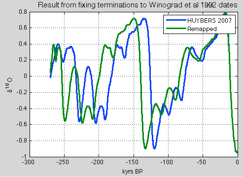
Figure 1
The method is basically a linear remapping. I’m sure there are better ways, but I don’t expect they would have a material impact on the outcome.
One point that’s important (with my very simple method) is the oldest agemarker we consider can cause an inconsistency (as there is nothing to constrain the dates between the last agemarker and the end date), which is why the first set below uses 270 kyrs.
T- III is dated by Winograd 1992 at 253 kyrs. So I picked a date shortly after that.
Here is the comparison of rate of change of ice volume with insolation, with the same conventions as in the last article. We can see that everything is nicely anti-correlated:

Figure 2 – Click to Expand
For comparison, the result (in the last article) from 0-200 kyrs BP without remapping the proxy dataset. We can see that everything is nicely correlated:
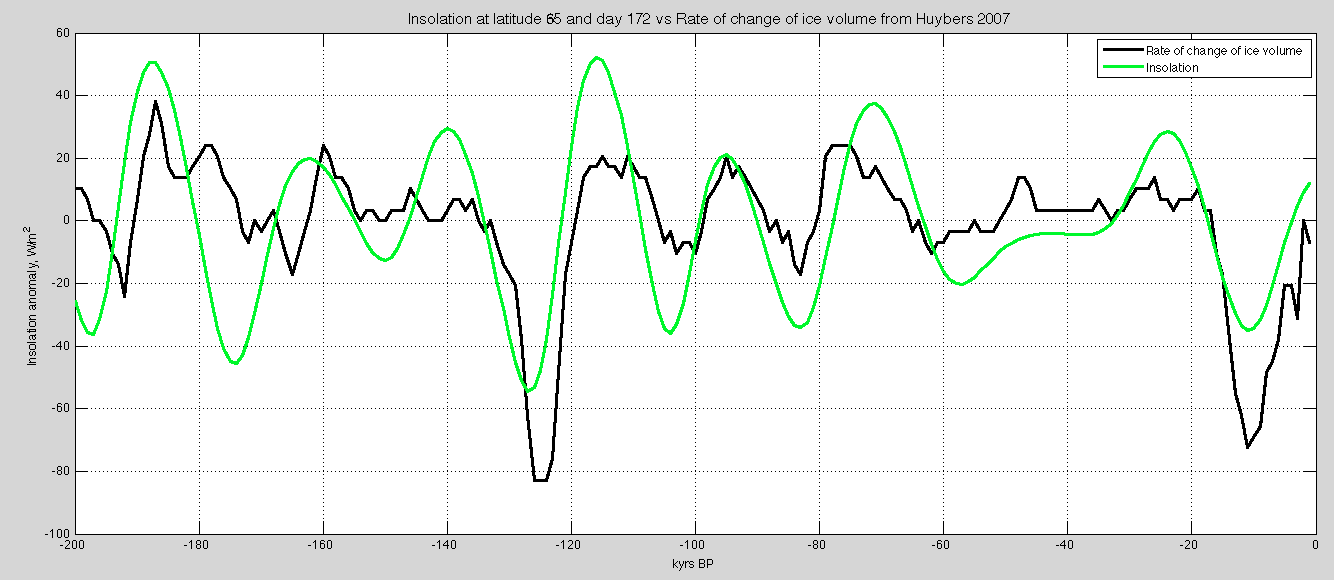
Figure 3 – Click to Expand
For the remapped data: correlation = -0.30. This is as negatively correlated to the insolation value as LR04 (an “orbitally-tuned” dataset) is positively correlated.
For interest I did the same exercise with a 0 – 200kyr BP timebase. This means everything from 140 kyrs – 200 yrs was not constrained by a revised T-III date. The result: correlation = 0. The interpretation is simple – the older data is not pulled out of alignment due to a later objective T-III date, so there is a better match of insolation with rate of change of ice volume for this older data.
Conclusion
Is there a conclusion? It’s surely staring us in the face so is left as an exercise for the interested student.
I have a headache.
Articles in the Series
Part One – An introduction
Part Two – Lorenz – one point of view from the exceptional E.N. Lorenz
Part Three – Hays, Imbrie & Shackleton – how everyone got onto the Milankovitch theory
Part Four – Understanding Orbits, Seasons and Stuff – how the wobbles and movements of the earth’s orbit affect incoming solar radiation
Part Five – Obliquity & Precession Changes – and in a bit more detail
Part Six – “Hypotheses Abound” – lots of different theories that confusingly go by the same name
Part Seven – GCM I – early work with climate models to try and get “perennial snow cover” at high latitudes to start an ice age around 116,000 years ago
Part Seven and a Half – Mindmap – my mind map at that time, with many of the papers I have been reviewing and categorizing plus key extracts from those papers
Part Eight – GCM II – more recent work from the “noughties” – GCM results plus EMIC (earth models of intermediate complexity) again trying to produce perennial snow cover
Part Nine – GCM III – very recent work from 2012, a full GCM, with reduced spatial resolution and speeding up external forcings by a factors of 10, modeling the last 120 kyrs
Part Ten – GCM IV – very recent work from 2012, a high resolution GCM called CCSM4, producing glacial inception at 115 kyrs
Pop Quiz: End of An Ice Age – a chance for people to test their ideas about whether solar insolation is the factor that ended the last ice age
Eleven – End of the Last Ice age – latest data showing relationship between Southern Hemisphere temperatures, global temperatures and CO2
Twelve – GCM V – Ice Age Termination – very recent work from He et al 2013, using a high resolution GCM (CCSM3) to analyze the end of the last ice age and the complex link between Antarctic and Greenland
Thirteen – Terminator II – looking at the date of Termination II, the end of the penultimate ice age – and implications for the cause of Termination II
Fourteen – Concepts & HD Data – getting a conceptual feel for the impacts of obliquity and precession, and some ice age datasets in high resolution
Fifteen – Roe vs Huybers – reviewing In Defence of Milankovitch, by Gerard Roe
Seventeen – Proxies under Water I – explaining the isotopic proxies and what they actually measure
Eighteen – “Probably Nonlinearity” of Unknown Origin – what is believed and what is put forward as evidence for the theory that ice age terminations were caused by orbital changes
Nineteen – Ice Sheet Models I – looking at the state of ice sheet models
References
In defense of Milankovitch, Gerard Roe, Geophysical Research Letters (2006) – free paper
Glacial variability over the last two million years: an extended depth-derived agemodel, continuous obliquity pacing, and the Pleistocene progression, Peter Huybers, Quaternary Science Reviews (2007) – free paper
Datasets for Huybers 2007 are here:
ftp://ftp.ncdc.noaa.gov/pub/data/paleo/contributions_by_author/huybers2006/
and
http://www.people.fas.harvard.edu/~phuybers/Progression/
Continuous 500,000-Year Climate Record from Vein Calcite in Devils Hole, Nevada, Winograd, Coplen, Landwehr, Riggs, Ludwig, Szabo, Kolesar & Revesz, Science (1992) – paywall, but might be available with a free Science registration
Insolation data calculated from Jonathan Levine’s MATLAB program
Notes
Note 1:
Here is an extract from Parennin et al 2007, The EDC3 chronology for the EPICA Dome C ice core:
In this article, we present EDC3, the new 800 kyr age scale of the EPICA Dome C ice core, which is generated using a combination of various age markers and a glaciological model. It is constructed in three steps.
First, an age scale is created by applying an ice flow model at Dome C. Independent age markers are used to control several poorly known parameters of this model (such as the conditions at the base of the glacier), through an inverse method.
Second, the age scale is synchronised onto the new Greenlandic GICC05 age scale over three time periods: the last 6 kyr, the last deglaciation, and the Laschamp event (around 41 kyr BP).
Third, the age scale is corrected in the bottom ∼500 m (corresponding to the time period 400–800 kyr BP), where the model is unable to capture the complex ice flow pattern..

From Parennin et al 2007


I can’t see any conclusion other than maybe the Devils hole data is not so accurate after all. If one assumes the Devils hole data is more objective, one could possibly say it looks like there is an orbital link to the glaciation cycles, but not in accordance with the Millankovich theory. Except for the problem that the most recent deglaciation would be an outlier. Hopefully a brighter student can draw a conclusion.
I’ll guess now that John has broken the ice. The conclusion is that the age dating of the paleo record is not certain enough to know whether or not the orbital cycles correlate with glacial terminations.
http://link.springer.com/chapter/10.1007/978-1-4419-9118-8_10
[…] 2014/02/03: TSoD: Ghosts of Climates Past — Sixteen — Roe vs Huybers II […]
Calling data conversion gurus. Hope someone can help.
I have the GISS d18O ocean database from http://data.giss.nasa.gov/o18data/ – file can be downloaded from this page – it is in the helpful format of:
Last time I had fixed text width files (HITRAN or CFC database) I spent literally 1-2 days working out the minutiae of Matlab textscan or some other command. It was very painful and this time around I don’t have a day or two to focus on data conversion minutiae. But for someone familiar with the process it is probably very quick.
This time I am hoping someone can help. I did manage to import the .txt file into Excel:
1. deleted the last two columns of Notes and Reference (because a blank Notes doesn’t get converted into a blank column, instead “Reference” becomes “Notes” and when both exist they turn into 2 columns – not at all necessary to fix this for the purposes of data evaluation).
2. converted the mthyear column that Excel brought in (because it read the text as a 5 or 6 character record instead of a 2 char/4 char record), into a separate month and year (using excel commands – right, left and len)
3. deleted values with year = “-999” – no idea of year so not much use
4. turned month 13 into blanks – maybe we want to use these, maybe not
5. turned values of salinity and temperature that were -999 into blanks
6. deleted d18O values that were -999 because that is the value we want so no value here
7. “converted” “general” format into “number” format – one of the excel minefields I think.
Great, I was thinking, this only took 45 minutes – then I did a MATLAB import of the resulting Excel and most of the values turned into NaN (not a number).
I remember this from some time ago. No idea how to fix this.
Can anyone assist? Calling date conversion gurus, or someone with the patience of a saint..
SoD,
The conversion seems to go very easily, when Excel reads all the text in the first column and the selection “Text to columns” is used to split the lines selecting “Fixed width” as the first choice and the right column widths on the next step.
The resulting sheet should be saved either as csv or tab delimited text file.
All that takes about 1 min.
Importing the data directly to Matlab seems to be equally easy and proceed with almost identical steps. The main thing to notice is adding a column splitter between the month and the year. Less important is the splitter after 15 characters of the “notes”, and removing all splitters within the references column.
One more comment on the NaNs.
They are probably due to Excel’s tendency to fill empty space sometimes by something that looks blank, but is not exactly that. I have removed such space by copying one such character to clipboard and using “Replace” to replace all such characters by nothing.
Thanks very much Pekka, you data conversion guru.
I had not realized I had those options in Excel.
Instead of removing the -999s and converting month 13 to blank I realize I can do it easier in Matlab without the risk of Excel turning a blank into a text item or something else.
So I followed your steps, created a .csv instead of Excel, imported into Matlab and all is fine.
Appreciate the help.
FWIW as a general rule rates in noisy data are inherently untrustworthy which is one reason Eli stays out of the rate of warming wars but, of course the variation due to the interplay of the various orbital parameters is interesting and to an extent an unsolved problem
There are all sorts of tricks to get decent rate estimates from noisy data, cubic splines comes to mind. The real trick is integrating noisy data, such as accelerometer and rotation rate readings to get velocity, position and orientation. Integrating noise gives you a random walk. The only cure is to have an independent reference measurement such as GPS position, velocity and heading to keep the integrated data from wandering off into never never land. But GPS data rates are too low to do things like flight control, which is why integrating accelerometer and rotation rate data is necessary in the first place. A three axis magnetometer is nice too, especially if you’re trying to control a helicopter. GPS only give you heading information when you’re moving. Note that all modern smart phones have the capability of performing these measurements.
The other alternative is to use low noise accelerometers like spinning precision machined beryllium spheres or ring laser gyros, but those are extremely expensive.
[…] Sixteen – Roe vs Huybers II – remapping a deep ocean core dataset and updating the previous article […]
[…] I’ll use the same temperature proxy dataset used in the discussion by Science of Doom here and here, which is the Huybers ∂18O dataset . For the insolation, I’m using the same Berger dataset […]