Feeds:
Posts
Comments

Archive for June, 2011

A long time ago I started writing this article. I haven’t yet finished it.

I realized that trying to write it was difficult because the audience criticism was so diverse. Come to me you huddled masses.. This paper, so simple in concept, has become somehow the draw card for “everyone against AGW”. The reasons why are not clear, since the paper is nothing to do with that.

As I review the “critiques” around the blogosphere, I don’t find any consistent objection. That makes it very hard to write about.

So, the reason for posting a half-finished article is for readers to say what they don’t agree with and maybe – if there is a consistent message/question – I will finish the article, or maybe answer the questions here. If readers think that the ideas in the paper somehow violate the first or second law of thermodynamics, please see note 1 and comment in those referenced articles. Not here.

==== part written article ===

In 1997, J. T. Kiehl and Kevin Trenberth’s paper was published, Earth’s Annual Global Mean Energy Budget. (Referred to as KT97 for the rest of this article).

For some reason it has become a very unpopular paper, widely criticized, and apparently viewed as “the AGW paper”.

This is strange as it is a paper which says nothing about AGW, or even possible pre-feedback temperature changes from increases in the inappropriately-named “greenhouse” gases.

KT97 is a paper which attempts to quantify the global average numbers for energy fluxes at the surface and the top of atmosphere. And to quantify the uncertainty in these values.

Of course, many people criticizing the paper believe the values violates the first or second law of thermodynamics. I won’t comment in the main article on the basic thermodynamics laws – for this, check out the links in note 1.

In this article I will try and explain the paper a little.  There are many updates from various researchers to the data in KT97, including Trenberth & Kiehl themselves (Trenberth, Fasullo and Kiehl 2009), with later and more accurate figures.

We are looking at this earlier paper because it has somehow become such a focus of attention.

Most people have seen the energy budget diagram as it appears in the IPCC TAR report (2001), but here it is reproduced for reference:

From Kiehl & Trenberth (1997)

From Kiehl & Trenberth (1997)

History and Utility

Many people have suggested that the KT97 energy budget is some “new invention of climate science”. And at the other end of the spectrum at least one commenter I read was angered by the fact that KT97 had somehow claimed this idea for themselves when many earlier attempts had been made long before KT97.

The paper states:

There is a long history of attempts to construct a global annual mean surface–atmosphere energy budget for the earth. The first such budget was provided by Dines (1917).

Compared with “imagining stuff”, reading a paper is occasionally helpful. KT97 is simply updating the field with the latest data and more analysis.

What is an energy budget?

It is an attempt to identify the relative and absolute values of all of the heat transfer components in the system under consideration. In the case of the earth’s energy budget, the main areas of interest are the surface and the “top of atmosphere”.

Why is this useful?

Well, it won’t tell you the likely temperature in Phoenix next month, whether it will rain more next year, or whether the sea level will change in 100 years.. but it helps us understand the relative importance of the different heat transfer mechanisms in the climate, and the areas and magnitude of uncertainty.

For example, the % of reflected solar radiation is now known to be quite close to 30%. That equates to around 103 W/m² of solar radiation (see note 2) that is not absorbed by the climate system. Compared with the emission of radiation from the earth’s climate system into space – 239 W/m² – this is significant. So we might ask – how much does this reflected % change? How much has it changed in the past? See The Earth’s Energy Budget – Part Four – Albedo.

In a similar way, the measurements of absorbed solar radiation and emitted thermal radiation into space are of great interest – do they balance? Is the climate system warming or cooling? How much uncertainty do we have about these measurements.

The subject of the earth’s energy budget tries to address these kind of questions and therefore it is a very useful analysis.

However, it is just one tiny piece of the jigsaw puzzle called climate.

Uncertainty

It might surprise many people that KT97 also say:

Despite these important improvements in our understanding, a number of key terms in the energy budget remain uncertain, in particular, the net absorbed shortwave and longwave surface fluxes.

And in their conclusion:

The purpose of this paper is not so much to present definitive values, but to discuss how they were obtained and give some sense of the uncertainties and issues in determining the numbers.

It’s true. There are uncertainties and measurement difficulties. Amazing that they would actually say that. Probably didn’t think people would read the paper..

AGW – “Nil points”

What does this paper say about AGW?

Nothing.

What does it say about feedback from water vapor, ice melting and other mechanisms?

Nothing.

What does it say about the changes in surface temperature from doubling of CO2 prior to feedback?

Nothing.

Top of Atmosphere

Since satellites started measuring:

  • incoming solar (shortware) radiation
  • reflected solar radiation
  • outgoing terrestrial (longwave) radiation

– it has become much easier to understand – and put boundaries around – the top of atmosphere (TOA) energy budget.

The main challenge is the instrument uncertainty. So KT97 consider the satellite measurements. The most accurate results available (at that time) were from five years of ERBE data (1985-1989).

From those results, the outgoing longwave radiation (OLR) from ERBE averaged 235 W/m² while the absorbed solar radiation averaged 238 W/m². Some dull discussion of error estimates from earlier various papers follows. The main result being that the error estimates are in the order of 5W/m², so it isn’t possible to pin down the satellite results any closer than that.

KT97 concludes:

Based on these error estimates, we assume that the bulk of the bias in the ERBE imbalance is in the shortwave absorbed flux at the top of the atmosphere, since the retrieval of shortwave flux is more sensitive than the retrieval of longwave flux to the sampling and modeling of the diurnal cycle, surface and cloud inhomogeneities.

Therefore, we use the ERBE outgoing longwave flux of 235 W/m² to define the absorbed solar flux.

What are they saying? That – based on the measurements and error estimates – a useful working assumption is that the earth (over this time period) is in energy balance and so “pick the best number” to represent that. Reflected solar radiation is the hardest to measure accurately (because it can be reflected in any direction) so we assume that the OLR is the best value to work from.

If the absorbed solar radiation and the OLR had been, say, 25 W/m² apart then the error estimates couldn’t have bridged this gap. And the choices would have been:

  • the first law of thermodynamics was wrong (150 years of work proven wrong)
  • the earth was cooling (warming) – depending on the sign of the imbalance
  • a mystery source of heating/cooling hadn’t been detected
  • one or both of the satellites was plain wrong (or the error estimates had major mistakes)

So all the paper is explaining about the TOA results is that the measurement results don’t justify concluding that the earth is out of energy balance and therefore they pick the best number to represent the TOA fluxes. That’s it. This shouldn’t be very controversial.

And also note that during this time period the ocean heat content (OHC) didn’t record any significant increase, so an assumption of energy balance during this period is reasonable.

And, as with any review paper, KT97 also include the results from previous studies, explaining where they agree and where they differ and possible/probable reasons for the differences.

In their later update of their paper (2009) they use the results of a climate model for the TOA imbalance. This comes to 0.9 W/m². In the context of the uncertainties they discuss this is not so significant. It is simply a matter of whether the TOA fluxes balance or not. This is something that is fundamentally unknown over a given 5-year or decadal time period.

As an exercise for the interested student, if you review KT97 with the working assumption that the TOA fluxes are out of balance by 1W/m², what changes of note take place to the various values in the 1997 paper?

Surface Fluxes

This is the more challenging energy balance. At TOA we have satellites measuring the radiation quite comprehensively – and we have only radiation as the heat transfer mechanism for incoming and outgoing energy.

At the surface the measurement systems are less complete. Why is that?

Firstly, we have movement of heat from the surface via latent heat and sensible heat – as well as radiation.

Secondly, satellites can only measure only a small fraction of the upward emitted surface radiation and none of the downward radiation at the surface.

Surface Fluxes – Radiation

To calculate the surface radiation, upward and downward, we need to rely on theory, on models.

You mean made up stuff that no one has checked?

Well, that’s what you might think if you read a lot of blogs that have KT97 on their hit list. It’s easy to make claims.

In fact, if we want to know on a global annual average basis what the upward and downward longwave fluxes are, and if we want to know the solar (shortwave) fluxes that reach the surface (vs absorbed in the atmosphere), we need to rely on models. This is simply because we don’t have 1,000’s of high quality radiation-measuring stations.

Instead we do have a small network of high-quality monitoring stations for measuring downward radiation – the BSRN (baseline surface radiation network) was established by the World Climate Research Programme (WCRP) in the early 1990’s. See The Amazing Case of “Back Radiation”.

The important point is that, for the surface values of downward solar and downward longwave radiation we can check the results of theory against measurements in the places where measurements are available. This tells us whether models are accurate or not.

To calculate the values of surface fluxes with the resolution to calculate the global annual average we need to rely on models. For many people, their instinctive response is that obviously this is not accurate. Instinctive responses are not science, though.

Digression – Many Types of Models

There are many different types of models. For example, if we want to know the value of the DLR (downward longwave radiation) at the surface on Nov 1st, 2210 we need to be sure that some important parameters are well-known for this date. We would need to know the temperature of the atmosphere as a function of height through the atmosphere – and also the concentration of CO2, water vapor, methane – and so on. We would need to predict all of these values successfully for Nov 1st, 2210.

The burden of proof is quite high for this “prediction”.

However, if we want to know the average value of DLR for 2009 we need to have a record of these parameters at lots of locations and times and we can do a proven calculation for DLR at these locations and times.

An Analogy – It isn’t much different from calculating how long the water will take to boil on the stove – we need to know how much water, the initial temperature of the water, the atmospheric temperature and what level you turned the heat to. If we want to predict this value for the future we will need to know what these values will be in the future. But to calculate the past is easy – if we already have a record of these parameters.

See Theory and Experiment – Atmospheric Radiation for examples of verifying theory against experiment.

End of Digression

And if we want to know the upward fluxes we need to know the reflected portion.

Related Articles

Kiehl & Trenberth and the Atmospheric Window

The Earth’s Energy Budget – Part One – a few climate basics.

The Earth’s Energy Budget – Part Two –  the important concept of energy balance at top of atmosphere.

References

Earth’s Annual Global Mean Energy Budget, Kiehl & Trenberth, Bulletin of the American Meteorological Society (1997) – free paper

Earth’s Global Energy Budget, Trenberth, Fasullo & Kiehl, Bulletin of the American Meteorological Society (2009) – free paper

Notes

Note 1 – The First Law of Thermodynamics is about the conservation of energy. Many people believe that because the temperature is higher at the surface than the top of atmosphere this somehow violates this first law. Check out Do Trenberth and Kiehl understand the First Law of Thermodynamics? as well as the follow-on articles.

The Second Law of Thermodynamics is about entropy increasing, due to heat flowing from hotter to colder. Many have created an imaginary law which apparently stops energy from radiation from a colder body being absorbed by a hotter body. Check out these articles:

Amazing Things we Find in Textbooks – The Real Second Law of Thermodynamics

The Three Body Problem

Absorption of Radiation from Different Temperature Sources

The Amazing Case of “Back Radiation” – Part Three and Part One and Part Two

Note 2 – When comparing solar radiation with radiation emitted by the climate system there is a “comparison issue” that has to be taken into account. Solar radiation is “captured” by an area of πr² (the area of a disc) because the solar radiation comes from a point source a long way away. But terrestrial radiation is emitted over the whole surface of the earth, an area of 4πr². So if we are talking about W/m² either we need to multiply terrestrial radiation by a factor of 4 to equate the two, or divide solar radiation by a factor of 4 to equate the two. The latter is conventionally chosen.

More about this in The Earth’s Energy Budget – Part One

Read Full Post »

During a discussion following one of the six articles on Ferenc Miskolczi someone pointed to an article in E&E (Energy & Environment). I took a look and had a few questions.

The article is question is The Thermodynamic Relationship Between Surface Temperature And Water Vapor Concentration In The Troposphere, by William C. Gilbert from 2010. I’ll call this WG2010. I encourage everyone to read the whole paper for themselves.

Actually this E&E edition is a potential collector’s item because they announce it as: Special Issue – Paradigms in Climate Research.

The author comments in the abstract:

 The key to the physics discussed in this paper is the understanding of the relationship between water vapor condensation and the resulting PV work energy distribution under the influence of a gravitational field.

Which sort of implies that no one studying atmospheric physics has considered the influence of gravitational fields, or at least the author has something new to offer which hasn’t previously been understood.

Physics

Note that I have added a WG prefix to the equation numbers from the paper, for ease of referencing:

First let’s start with the basic process equation for the first law of thermodynamics
(Note that all units of measure for energy in this discussion assume intensive properties, i.e., per unit mass):

dU = dQ – PdV ….[WG1]

where dU is the change in total internal energy of the system, dQ is the change in thermal energy of the system and PdV is work done to or by the system on the surroundings.

This is (almost) fine. The author later mixes up Q and U. dQ is the heat added to the system. dU is change in internal energy which includes the thermal energy.

But equation (1) applies to a system that is not influenced by external fields. Since the atmosphere is under the influence of a gravitational field the first law equation must be modified to account for the potential energy portion of internal energy that is due to position:

dU = dQ + gdz – PdV ….[WG2]

where g is the acceleration of gravity (9.8 m/s²) and z is the mass particle vertical elevation relative to the earth’s surface.

[Emphasis added. Also I changed “h” into “z” in the quotes from the paper to make the equations easier to follow later].

This equation is incorrect, which will be demonstrated later.

The thermal energy component of the system (dQ) can be broken down into two distinct parts: 1) the molecular thermal energy due to its kinetic/rotational/ vibrational internal energies (CvdT) and 2) the intermolecular thermal energy resulting from the phase change (condensation/evaporation) of water vapor (Ldq). Thus the first law can be rewritten as:

dU = CvdT + Ldq + gdz – PdV ….[WG3]

where Cv is the specific heat capacity at constant volume, L is the latent heat of condensation/evaporation of water (2257 J/g) and q is the mass of water vapor available to undergo the phase change.

Ouch. dQ is heat added to the system, and it is dU which is the internal energy which should be broken down into changes in thermal energy (temperature) and changes in latent heat. This is demonstrated later.

Later, the author states:

This ratio of thermal energy released versus PV work energy created is the crux of the physics behind the troposphere humidity trend profile versus surface temperature. But what is it that controls this energy ratio? It turns out that the same factor that controls the pressure profile in the troposphere also controls the tropospheric temperature profile and the PV/thermal energy ratio profile. That factor is gravity. If you take equation (3) and modify it to remove the latent heat term, and assume for an adiabatic, ideal gas system CpT = CvT + PV, you can easily derive what is known in the various meteorological texts as the “dry adiabatic lapse rate”:

dT/dz = –g/Cp = 9.8 K/km ….[WG5]

[Emphasis added]

Unfortunately, with his starting equations you can’t derive this result.

What I am talking about?

The Equations Required to Derive the Lapse Rate

Most textbooks on atmospheric physics include some derivation of the lapse rate. We consider a parcel of air of one mole. (Some terms are defined slightly differently to WG2010 – note 1).

There are 5 basic equations:

The hydrostatic equilibrium equation:

dp/dz = -ρg ….[1]

where p = pressure, z = height, ρ = density and g = acceleration due to gravity (=9.8 m/s²)

The ideal gas law:

pV = RT ….[2]

where V = volume, R = the gas constant, T = temperature in K, and this form of the equation is for 1 mole of gas

The equation for density:

ρ = M/V ….[3]

where M = mass of one mole

The First Law of Thermodynamics:

dU = dQ + dW ….[4]

where dU = change in internal energy, dQ = heat added to the system, dW = work added to the system

..rewritten for dry atmospheres as:

dQ = CvdT + pdV ….[4a]

where Cv = heat capacity at constant volume (for one mole), dV = change in volume

And the (less well-known) equation which links heat capacity at constant volume with heat capacity at constant pressure (derived from statistical thermodynamics and experimentally verifiable):

Cp = Cv + R ….[5]

where Cp = heat capacity (for one mole) at constant pressure

With an adiabatic process no heat is transferred between the parcel and its surroundings. This is a reasonable assumption with typical atmospheric movements. As a result, we set dQ = 0 in equation 4 & 4a.

Using these 5 equations we can solve to find the dry adiabatic lapse rate (DALR):

dT/dz = -g/cp ….[6]

where dT/dz = the change in temperature with height (the lapse rate), g = acceleration due to gravity, and cp = specific heat capacity (per unit mass) at constant pressure

dT/dz ≈ -9.8 K/km

Knowing that many readers are not comfortable with maths I show the derivation in The Maths Section at the end.

And also for those not so familiar with maths & calculus, the “d” in front of a term means “change in”. So, for example, “dT/dz” reads as: “the change in temperature as z changes”.

Fundamental “New Paradigm” Problems

There are two basic problems with his fundamental equations:

  • he confuses internal energy and heat added to get a sign error
  • he adds a term for gravitational potential energy when it is already implicitly included via the pressure change with height

A sign error might seem unimportant but given the claims later in the paper (with no explanation of how these claims were calculated) it is quite possible that the wrong equation was used to make these calculations.

These problems will now be explained.

Under the New Paradigm – Sign Error

Because William Gilbert mixes up internal energy and heat added, the result is a sign error. Consult a standard thermodynamics textbook and the first law of thermodynamics will be represented something like this:

dU = dQ + dW

Which in words means:

The change in internal energy equals the heat added plus the work done on the system.

And if we talk about dW as the work done by the system then the sign in front of dW will change. So, if we rewrite the above equation:

dU = dQ – pdV

By the time we get to [WG3] we have two problems.

Here is [WG3] for reference:

dU = CvdT + Ldq + gdz – PdV ….[WG3]

The first problem is that for adiabatic process, no heat is added to (or removed from) the system. So dQ = 0. The author says dU = 0 and makes dQ = change in internal energy (=CvdT + Ldq).

Here is the demonstration of the problem using his equation..

If we have no phase change then Ldq = 0. The gdz term is a mistake – for later consideration – but if we consider an example with no change in height in the atmosphere, we would have (using his equation):

CvdT – PdV = 0 ….[WG3a]

So if the parcel of air expands, doing work on its environment, what happens to temperature?

dV is positive because the volume is increasing. So to keep the equation valid, dT must be positive, which means the temperature must increase.

This means that as the parcel of air does work on its environment, using up energy, its temperature increases – adding energy. A violation of the first law of thermodynamics.

Hopefully, everyone can see that this is not correct. But it is the consequence of the incorrectly stated equation. In any case, I will use both the flawed and the fixed version to demonstrate the second problem.

Under the New Paradigm – Gravity x 2

This problem won’t appear so obvious, which is probably why William Gilbert makes the mistake himself.

In the list of 5 equations, I wrote:

dQ = CvdT + pdV ….[4a]

This is for dry atmospheres, to keep it simple (no Ldq term for water vapor condensing). If you check the Maths Section at the end, you can see that using [4a] we get the result that everyone agrees with for the lapse rate.

I didn’t write:

dQ = CvdT + Mgdz + pdV ….[should this instead be 4a?]

[Note that my equations consider 1 mole of the atmosphere rather than 1 kg which is why “M” appears in front of the gdz term].

So how come I ignored the effect of gravity in the atmosphere yet got the correct answer? Perhaps the derivation is wrong?

The effect of gravity already shows itself via the increase in pressure as we get closer to the surface of the earth.

Atmospheric physics has not been ignoring the effect of gravity and making elementary mistakes. Now for the proof.

If you consult the Maths Section, near the end we have reached the following equation and not yet inserted the equation for the first law of thermodynamics:

pdV – Mgdz = (Cp-Cv)dT ….[10]

Using [10] and “my version” of the first law I successfully derive dT/dz = -g/cp (the right result). Now we will try using William Gilbert’s equation [WG3], with Ldq = 0, to derive the dry adiabatic lapse rate.

0 = CvdT + gdz – PdV ….[WG3b]

and rewriting for one mole instead of 1 kg (and using my terms, see note 1):

pdV = CvdT + Mgdz ….[WG3c]

Inserting WG3c into [10]:

CvdT + Mgdz – Mgdz = (Cp-Cv)dT ….[11]

which becomes:

Cv = (Cp-Cv) ↠   Cp = Cv/2 ….[11a]

A New Paradigm indeed!

Now let’s fix up the sign error in WG3 and see what result we get:

0 = CvdT + gdz + PdV ….[WG3d]

and again rewriting for one mole instead of 1 kg (and again using my terms, see note 1):

pdV = -CvdT – Mgdz ….[WG3e]

Inserting WG3e into [10]:

-CvdT – Mgdz – Mgdz = (Cp-Cv)dT ….[12]

which becomes:

-CvdT – 2Mgdz = CpdT – CvdT ….[12a]

and canceling the -CvdT term from each side:

-2Mgdz = CpdT ….[12b]

So:

dT/dz = -2Mg/Cp, and because specific heat capacity, cp = Cp/M

dT/dz = -2g/cp ….[12c]

The result of “correctly including gravity” is that the dry adiabatic lapse rate ≈ -19.6 K/km. 

Note the factor of 2. This is because we are now including gravity twice. The pressure in the atmosphere reduces as we go up – this is because of gravity. When a parcel of air expands due to its change in height, it does work on its surroundings and therefore reduces in temperature  – adiabatic expansion. Gravity is already taken into account with the hydrostatic equation.

The Physics of Hand-Waving

The author says:

As we shall see, PV work energy is very important to the understanding of this thermodynamic behavior of the atmosphere, and the thermodynamic role of water vapor condensation plays an important part in this overall energy balance. But this is unfortunately often overlooked or ignored in the more recent climate science literature. The atmosphere is a very dynamic system and cannot be adequately analyzed using static, steady state mental models that primarily focus only on thermal energy.

Emphasis added. This is an unproven assertion because it comes with no references.

In the next stage of the “physics” section, the author doesn’t bother with any equations, making it difficult to understand exactly what he is claiming.

Keeping this gravitational steady state equilibrium in mind, let’s look again at what happens when latent heat is released (condensation) during air parcel ascension.

Latent heat release immediately increases the parcel temperature. But that also results in rapid PV expansion which then results in a drop in parcel temperature. Buoyancy results and the parcel ascends and is driven by the descending pressure profile created by gravity.

The rate of ascension, and the parcel temperature, is a function of the quantity of latent heat released and the PV work needed to overcome the gravitational field to reach a dynamic equilibrium. The more latent heat that is released, the more rapid the expansion / ascension. And the more rapid the ascension, the more rapid is the adiabatic cooling of the parcel. Thus the PV/thermal energy ratio should be a function of the amount of latent heat available for phase conversion at any given altitude. The corresponding physics shows the system will try to force the convecting parcel to approach the dry adiabatic or “gravitational” lapse rate as internal latent heat is released.

For the water vapor remaining uncondensed in the parcel, saturation and subsequent condensation will occur at a more rapid rate if more latent heat is released. In fact if the cooling rate is sufficiently large, super saturation can occur, which can then cause very sudden condensation in greater quantity. Thus the thermal/PV energy ratio is critical in determining the rate of condensation occurring. The higher this ratio, the more complete is the condensation in the parcel, and the lower the specific humidity will be at higher elevations.

I tried (unsuccessfully) to write down some equations to reflect the above paragraphs. The correct approach for the author would be:

  • A. Here is what atmospheric physics states now (with references)
  • B. Here are the flaws/omissions due to theoretical consideration i), ii), etc
  • C. Here is the new derivation (with clear statement of physics principles upon which the new equations are based)

One point I think the author is claiming is that the speed of ascent is a critical factor. Yet the equation for the moist adiabatic lapse rate doesn’t allow for a function of time in the equation.

The (standard) equation has the form (note 2):

dT/dz = g/cp {[1+Lq*/RT]/[1+βLq*/cp]} ….[13]

where q* is the saturation specific humidity and is a function of p & T (i.e. not a constant), and β = 0.067/°C. (See, for example: Atmosphere, Ocean & Climate Dynamics by Marshall & Plumb, 2008)

And this means that if the ascent is – for example – twice as fast, the amount of water vapor condensed at any given height will still be the same. It will happen in half the time, but why will this change any of the thermodynamics of the process?

It might, but it’s not clearly stated, so who can determine the “new physics”?

I can see that something else is claimed to do with the ratio CvdT /pV but I don’t know what it is, or what is behind the claim.

Writing the equations down is important so that other people can evaluate the claim.

And the final “result” of the hand waving is what appears to be the crux of the paper – more humidity at the surface will cause so much “faster” condensation of the moisture that the parcel of air will be drier higher up in the atmosphere. (Where “faster” could mean dT/dt, or could mean dT/dz).

Assuming I understood the claim of the paper correctly it has not been proven from any theoretical considerations. (And I’m not sure I have understood the claim correctly).

Empirical Observations

The heading is actually “Empirical Observations to Verify the Physics”. A more accurate title is “Empirical Observations”.

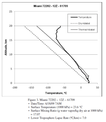
The author provides 3 radiosonde profiles from Miami. Here is one example:

From Gilbert (2010)

From Gilbert (2010)

Figure 1 – “Thermal adiabat” in the legend = “moist adiabat”

With reference to the 3 profiles, a higher surface humidity apparently leads to complete condensation at a lower altitude.

This is, of course, interesting. This would mean a higher humidity at the surface leads to a drier upper troposphere.

But it’s just 3 profiles. From one location on two different days. Does this prove something or should a few more profiles be used?

A few statements that need backing up:

The lower troposphere lapse rate decreases (slower rate of cooling) with increasing system surface humidity levels, as expected. But the differences in lapse rate are far less than expected based on the relative release of latent heat occurring in the three systems.

What equation determines “than expected”? What result was calculated vs measured? What implications result?

The amount of PV work that occurs during ascension increases markedly as the system surface humidity levels increase, especially at lower altitudes..

How was this calculated? What specifically is the claim? The equation 4a, under adiabatic conditions, with the additional of latent heat reads like this:

CvdT + Ldq + pdV = 0 ….[4a]

Was this equation solved from measured variables of pressure, temperature & specific humidity?

Latent heat release is effectively complete at 7.5 km for the highest surface humidity system (20.06 g/kg) but continues up to 11 km for the lower surface humidity systems (18.17 and 17.07 g/kg). The higher humidity system has seen complete condensation at a lower altitude, and a significantly higher temperature (−17 ºC) than the lower humidity systems (∼ −40 ºC) despite the much greater quantity of latent heat released.

How was this determined?

If it’s true, perhaps the highest humidity surface condition ascended into a colder air front and therefore lost all its water vapor due to the lower temperature?

Why is this (obvious) possibility not commented on or examined??

Textbook Stuff and Why Relative Humidity doesn’t Increase with Height

The radiosonde profiles in the paper are not necessarily following one “parcel” of air.

Consider a parcel of air near saturation at the surface. It rises, cools and soon reaches saturation. So condensation takes place, the release of latent heat causes the air to be more buoyant and so it keeps rising. As it rises water vapor is continually condensing and the air (of this parcel) will be at 100% relative humidity.

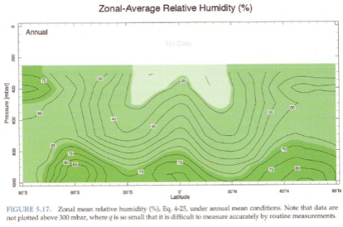
Yet relative humidity doesn’t increase with height, it reduces:

From Marshall & Plumb (2008)

From Marshall & Plumb (2008)

Figure 2

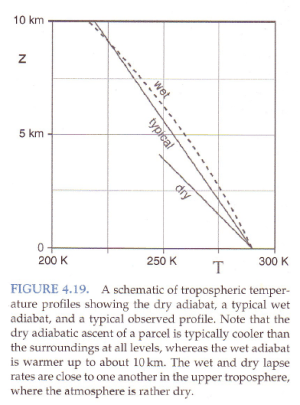
Standard textbook stuff on typical temperature profiles vs dry and moist adiabatic profiles:

From Marshall & Plumb (2008)

From Marshall & Plumb (2008)

Figure 3

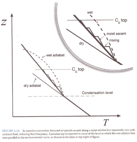
And explaining why the atmosphere under convection doesn’t always follow a moist adiabat:

From Marshall & Plumb (2008)

From Marshall & Plumb (2008)

Figure 4 

The atmosphere has descending dry air as well as rising moist air. Mixing of air takes place, which is why relative humidity reduces with height.

Conclusion

The “theory section” of the paper is not a theory section. It has a few equations which are incorrect, followed by some hand-waving arguments that might be interesting if they were turned into equations that could be examined.

It is elementary to prove the errors in the few equations stated in the paper. If we use the author’s equations we derive a final result which contradicts known fundamental thermodynamics.

The empirical results consist of 3 radiosonde profiles with many claims that can’t be tested because the method by which these claims were calculated is not explained.

If it turned out that – all other conditions remaining the same – higher specific humidity at the surface translated into a drier upper troposphere, this would be really interesting stuff.

But 3 radiosonde profiles in support of this claim is not sufficient evidence.

The Maths Section – Real Derivation of Dry Adiabatic Lapse Rate

There are a few ways to get to the final result – this is just one approach. Refer to the original 5 equations under the heading: The Equations for the Lapse Rate.

From [2], pV = RT, differentiate both sides with respect to T:

↠ d(pV)/dT = d(RT)/dT

The left hand side can be expanded as: V.dp/dT + p.dV/dT, and the right hand side = R (as dT/dT=1).

↠ Vdp + pdV = RdT  ….[7]

Insert [5], Cp = Cv + R, into [7]:

Vdp + pdV = (Cp-Cv)dT ….[8]

From [1] & [3]:

Vdp = -Mgdz ….[9]

Insert [9] into [8]:

pdV – Mgdz = (Cp-Cv)dT ….[10]

From 4a, under adiabatic conditions, dQ = 0, so CvdT + pdV = 0, and substituting into [10]”

-CvdT – Mgdz = CpdT – CvdT

and adding CvdT to both sides:

-Mgdz = CpdT, or dT/dz = -Mg/Cp ….[11]

and specific heat capacity, cp = Cp/M, so:

dT/dz = g /cp ….[11a]

The correct result, stated as equation [6] earlier.

Notes

Note 1: Definitions in equations. WG2010 has:

  • P = pressure, while this article has p = pressure (lower case instead of upper case0
  •  Cv = heat capacity for 1 kg, this article has Cv = heat capacity for one mole, and cv = heat capacity for 1 kg.

Note 2: The moist adiabatic lapse rate is calculated using the same approach but with an extra term, Ldq, in equation 4a, which accounts for the latent heat released as water vapor condenses.
Read Full Post »

In Part One we saw:

  • some trends based on real radiosonde measurements
  • some reasons why long term radiosonde measurements are problematic
  • examples of radiosonde measurement “artifacts” from country to country
  • the basis of reanalyses like NCEP/NCAR
  • an interesting comparison of reanalyses against surface pressure measurements
  • a comparison of reanalyses against one satellite measurement (SSMI)

But we only touched on the satellite data (shown in Trenberth, Fasullo & Smith in comparison to some reanalysis projects).

Wentz & Schabel (2000) reviewed water vapor, sea surface temperature and air temperature from various satellites. On water vapor they said:

..whereas the W [water vapor] data set is a relatively new product beginning in 1987 with the launch of the special sensor microwave imager (SSM/I), a multichannel microwave radiometer. Since 1987 four more SSM/I’s have been launched, providing an uninterrupted 12-year time series. Imaging radiometers before SSM/I were poorly calibrated, and as a result early water-vapour studies (7) were unable to address climate variability on interannual and decadal timescales.

The advantage of SSMI is that it measures the 22 GHz water vapor line. Unlike measurements in the IR around 6.7 μm (for example the HIRS instrument) which require some knowledge of temperature, the 22 GHz measurement is a direct reflection of water vapor concentration. The disadvantage of SSMI is that it only works over the ocean because of the low ocean emissivity (but variable land emissivity). And SSMI does not provide any vertical resolution of water vapor concentration, only the “total precipitable water vapor” (TPW) also known as “column integrated water vapor” (IWV).

The algorithm, verification and error analysis for the SSMI can be seen in Wentz’s 1997 JGR paper: A well-calibrated ocean algorithm for special sensor microwave / imager.

Here is Wentz & Schabel’s graph of IWV over time (shown as W in their figure):

From Wentz & Schabel (2000)

From Wentz & Schabel (2000)

Figure 1 – Region captions added to each graph

They calculate, for the short period in question (1988-1998):

  • 1.9%/decade for 20°N – 60°N
  • 2.1%/decade for 20°S – 20°N
  • 1.0%/decade for 20°S – 60°S

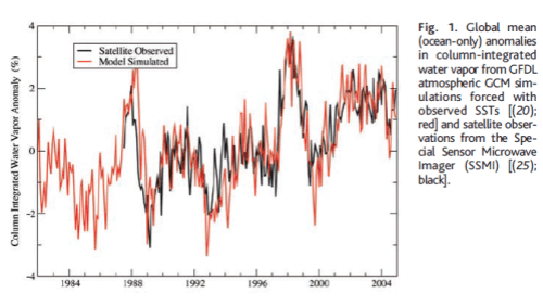
Soden et al (2005) take the dataset a little further and compare it to model results:

From Soden et al (2005)

From Soden et al (2005)

Figure 2

They note the global trend of 1.4 ± 0.78 %/decade.

As their paper is more about upper tropospheric water vapor they also evaluate the change in channel 12 of the HIRS instrument (High Resolution Infrared Radiometer Sounder):

The radiance channel centered at 6.7 μm (channel 12) is sensitive to water vapor integrated over a broad layer of the upper troposphere (200 to 500 hPa) and has been widely used for studies of upper tropospheric water vapor. Because clouds strongly attenuate the infrared radiation, we restrict our analysis to clear-sky radiances in which the upwelling radiation in channel 12 is not affected by clouds.

The change in radiance from channel 12 is approximately zero over the time period, which for technical reasons (see note 1) corresponds to roughly constant relative humidity in that region over the period from the early 1980’s to 2004. You can read the technical explanation in their paper, but as we are focusing on total water vapor (IWV) we will leave a discussion over UTWV for another day.

Updated Radiosonde Trends

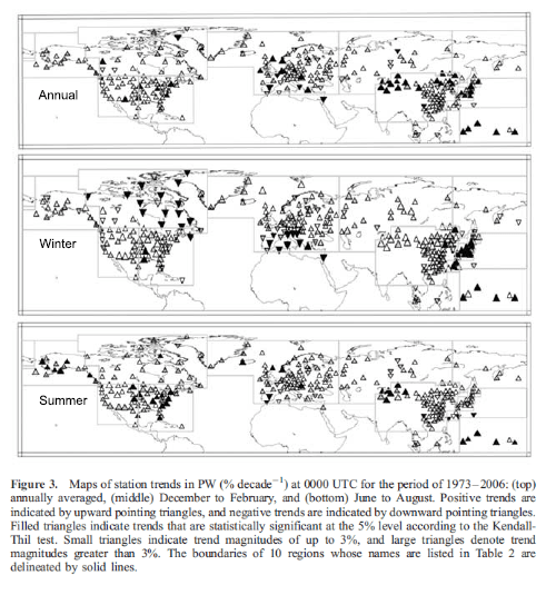
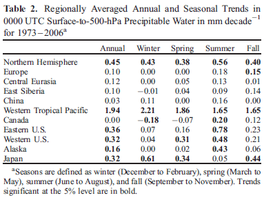
Durre et al (2009) updated radiosonde trends in their 2009 paper. There is a lengthy extract from the paper in note 2 (end of article) to give insight into why radiosonde data cannot just be taken “as is”, and why a method has to be followed to identify and remove stations with documented or undocumented instrument changes.

Importantly they note, as with Ross & Elliott 2001:

..Even though the stations were located in many parts of the globe, only a handful of those that qualified for the computation of trends were located in the Southern Hemisphere. Consequently, the trend analysis itself was restricted to the Northern Hemisphere as in that of RE01..

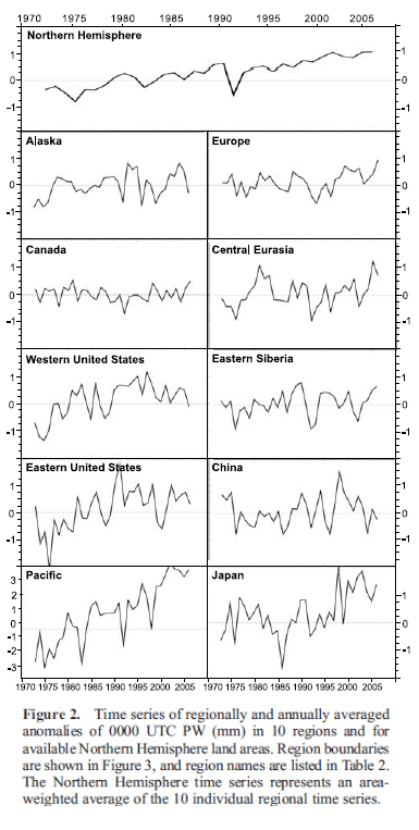
Here are their time-based trends:

From Durre et al (2009)

From Durre et al (2009)

Figure 3

And a map of trends:

From Durre et al (2009)

From Durre et al (2009)

Figure 4

Note the sparse coverage of the oceans and also the land regions in Africa and Asia, except China.

And their table of results:

From Durre et al (2009)

From Durre et al (2009)

Figure 5

A very interesting note on the effect of their removal of stations based on detection of instrument changes and other inhomogeneities:

Compared to trends based on unadjusted PW data (not shown), the trends in Table 2 are somewhat more positive. For the Northern Hemisphere as a whole, the unadjusted trend is 0.22 mm/decade, or 0.23 mm/decade less than the adjusted trend.

This tendency for the adjustments to yield larger increases in PW is consistent with the notion that improvements in humidity measurements and observing practices over time have introduced an artificial drying into the radiosonde record (e.g., RE01).

TOPEX Microwave

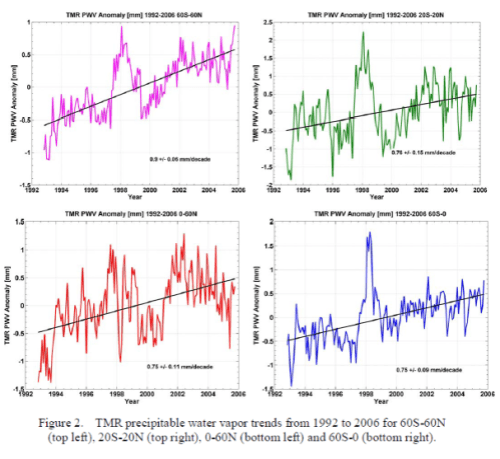
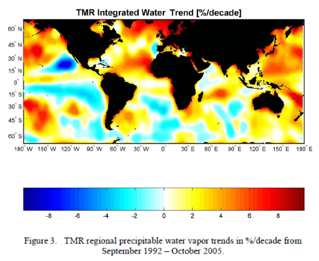
Brown et al (2007) evaluated data from the Topex Microwave Radiometer (TMR). This is included on the Topex/Poseiden oceanography satellite and is dedicated to measuring the integrated water vapor content of the atmosphere. TMR is nadir pointing and measures the radiometric brightness temperature at 18, 21 and 37 GHz. As with SSMI, it only provides data over the ocean.

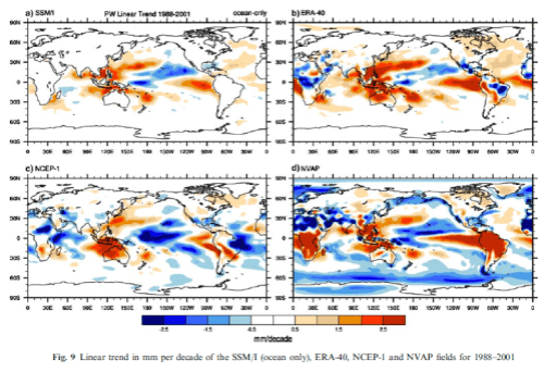
For the period of operation of the satellite (1992 – 2005) they found the trend of 0.90 ± 0.06 mm/decade:

From Brown et al (2007)

From Brown et al (2007)

Figure 6 – Click for a slightly larger view

And a map view:

From Brown et al (2007)

From Brown et al (2007)

Figure 7

Paltridge et al (2009)

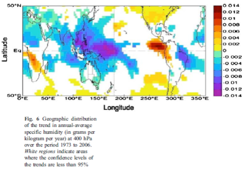
Paltridge, Arking & Pook (2009) – P09 – take a look at the NCEP/NCAR reanalysis project from 1973 – 2007. They chose 1973 as the start date for the reasons explained in Part One – Elliott & Gaffen have shown that pre-1973 data has too many problems. They focus on humidity data below 500mbar as the measurement of humidity at higher altitudes and lower temperatures are more prone to radiosonde problems.

The NCEP/NCAR data shows positive trends below 850 mbar (=hPa) in all regions, negative trends above 850 mbar in the tropics and midlatitudes, and negative trends above 600 mbar in the northern midlatitudes.

Here are the water vapor trends vs height (pressure) for both relative humidity and specific humidity:

From Paltridge et al (2009)

From Paltridge et al (2009)

Figure 8

And here is the map of trends:

from Paltridge et al (2009)

from Paltridge et al (2009)

Figure 9

They comment on the “boundary layer” vs “free troposphere” issue.. In brief the boundary layer is that “well-mixed layer” close to the surface where the friction from the ground slows down the atmospheric winds and results in more turbulence and therefore a well-mixed layer of atmosphere. This is typically around 300m to 1000m high (there is no sharp “cut off”). At the ocean surface the atmosphere tends to be saturated (if the air is still) and so higher temperatures lead to higher specific humidities. (See Clouds and Water Vapor – Part Two if this is a new idea). Therefore, the boundary layer is uncontroversially expected to increase its water vapor content with temperature increases. It is the “free troposphere” or atmosphere above the boundary layer where the debate lies.

They comment:

It is of course possible that the observed humidity trends from the NCEP data are simply the result of problems with the instrumentation and operation of the global radiosonde network from which the data are derived.

The potential for such problems needs to be examined in detail in an effort rather similar to the effort now devoted to abstracting real surface temperature trends from the face-value data from individual stations of the international meteorological networks.

In the meantime, it is important that the trends of water vapor shown by the NCEP data for the middle and upper troposphere should not be “written off” simply on the basis that they are not supported by climate models—or indeed on the basis that they are not supported by the few relevant satellite measurements.

There are still many problems associated with satellite retrieval of the humidity information pertaining to a particular level of the atmosphere— particularly in the upper troposphere. Basically, this is because an individual radiometric measurement is a complicated function not only of temperature and humidity (and perhaps of cloud cover because “cloud clearing” algorithms are not perfect), but is also a function of the vertical distribution of those variables over considerable depths of atmosphere. It is difficult to assign a trend in such measurements to an individual cause.

Since balloon data is the only alternative source of information on the past behavior of the middle and upper tropospheric humidity and since that behavior is the dominant control on water vapor feedback, it is important that as much information as possible be retrieved from within the “noise” of the potential errors.

So what has P09 added to the sum of knowledge? We can already see the NCEP/NCAR trends in Trends and variability in column-integrated atmospheric water vapor by Trenberth et al from 2005.

Did the authors just want to take the reanalysis out of the garage, drive it around the block a few times and park it out front where everyone can see it?

No, of course not!

– I hear all the NCEP/NCAR believers say.

One of our commenters asked me to comment on Paltridge’s reply to Dessler (which was a response to Paltridge..), and linked to another blog article. It seems like even the author of that blog article is confused about NCEP/NCAR. This reanalysis project (as explained in Part One), is a model output not a radiosonde dataset:

Humidity is in category B – ‘although there are observational data that directly affect the value of the variable, the model also has a very strong influence on the value ‘

And for those people who have a read of Kalnay’s 1996 paper describing the project they will see that with the huge amount of data going into the model, the data wasn’t quality checked by human inspection on the way in. Various quality control algorithms attempt to (automatically) remove “bad data”.

This is why we have reviewed Ross & Elliott (2001) and Durre et al (2009). These papers review the actual radiosonde data and find increasing trends in IWV. They also describe in a lot of detail what kind of process they had to go through to produce a decent dataset. The authors of both papers also both explained that they could only produce a meaningful trend for the northern hemisphere. There is not enough quality data for the southern hemisphere to even attempt to produce a trend.

And Durre et al note that when they use the complete dataset the trend is half that calculated with problematic data removed.

This is the essence of the problem with Paltridge et al (2009)

Why is Ross & Elliot (2001) not reviewed and compared? If Ross & Elliott found that Southern Hemisphere trends could not be calculated because of the sparsity of quality radiosonde data, why doesn’t P09 comment on that? Perhaps Ross & Elliott are wrong. But no comment from P09. (Durre et al find the same problem with SH data, and probably too late for P09 but not too late for the 2010 comments the authors have been making).

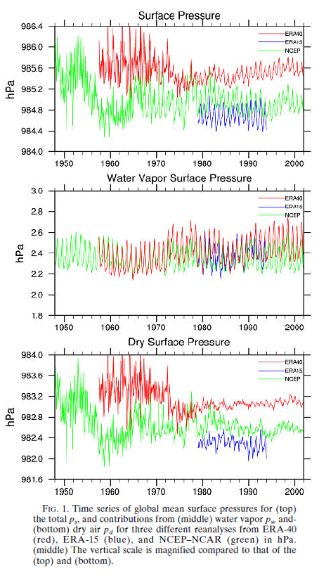
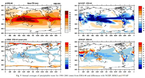
In The Mass of the Atmosphere: A Constraint on Global Analyses, Trenberth & Smith pointed out clear problems with NCEP/NCAR vs ERA-40. Perhaps Trenberth and Smith are wrong. Or perhaps there is another way to understand these results. But no comment on this from P09.

P09 comment on the issues with satellite humidity retrieval for different layers of the atmosphere but no comment on the results from the microwave SSMI which has a totally different algorithm to retrieve IWV. And it is important to understand that they haven’t actually demonstrated a problem with satellite measurements. Let’s review their comment:

In the meantime, it is important that the trends of water vapor shown by the NCEP data for the middle and upper troposphere should not be “written off” simply on the basis that they are not supported by climate models—or indeed on the basis that they are not supported by the few relevant satellite measurements.

The reader of the paper wouldn’t know that Trenberth & Smith have demonstrated an actual reason for preferring ERA-40 (if any reanalysis is to be used).

The reader of the paper might understand “a few relevant satellite measurements” as meaning there wasn’t much data from satellites. If you review figure 4 you can see that the quality radiosonde data is essentially mid-latitude northern hemisphere land. Satellites – that is, multiple satellites with different instruments at different frequencies – have covered the oceans much much more comprehensively than radiosondes. Are the satellites all wrong?

The reader of the paper would think that the dataset has been apparently ditched because it doesn’t fit climate models.

This is probably the view of Paltridge, Arking & Pook. But they haven’t demonstrated it. They have just implied it.

Dessler & Davis (2010)

Dessler & Davis responded to P09. They plot some graphs from 1979  to present. The reason for plotting graphs from 1979 is because this is when the satellite data was introduced. And all of the reanalysis projects, except NCEP/NCAR incorporated satellite humidity data. (NCEP/NCAR does incorporate satellite data for some other fields).

Basically when data from a new source is introduced, even if it is more accurate, it can introduce spurious trends and even in opposite direction to the real trends. This was explained in Part One under the heading Comparing Reanalysis of Humidity. So trend analysis usually takes place over periods of consistent data sources.

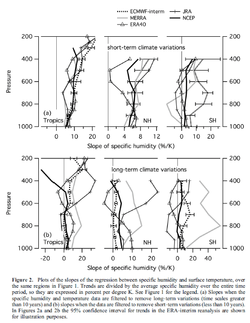
This figure contrasts short term relationships between temperature and humidity with long term relationships:

From Dessler & Davis (2010)

From Dessler & Davis (2010)

Figure 10

If the blog I referenced earlier is anything to go by, the primary reason for producing this figure has been missed. And as that blog article seemed to not comprehend that NCEP/NCAR is a reanalysis (= model output) it’s not so surprising.

Dessler & Davis said:

There is poorer agreement among the reanalyses, particularly compared to the excellent agreement for short‐term fluctuations. This makes sense: handling data inhomogeneities will introduce long‐term trends in the data but have less effect on short‐term trends. This is why long term trends from reanalyses tend to be looked at with suspicion [e.g., Paltridge et al., 2009; Thorne and Vose, 2010; Bengtsson et al., 2004].

[Emphasis added]

They are talking about artifacts of the model (NCEP/NCAR). In the short term the relationship between humidity and temperature agree quite well among the different reanalyses. But in the longer term NCEP/NCAR doesn’t – demonstrating that it is likely introducing biases.

The alternative, as Dessler & Davis explain, is that there is somehow an explanation for a long term negative feedback (temperature and water vapor) with a short term positive feedback.

If you look around the blog world, or at say, Professor Lindzen you don’t find this. You find arguments about why short term feedback is negative. Not an argument that short term is positive and yet long term is negative.

I agree that many people say:  “I don’t know, it’s complicated, perhaps there is a long term negative feedback..” and I respect that point of view.

But in the blog article pointed to me by our commenter in Part One, the author said:

JGR let some decidedly unscientific things slip into that Dessler paper. One of the reasons provided is nothing more than a form of argument from ignorance: “there’s no theory that explains why the short term might be different to the long term”.

Why would any serious scientist admit that they don’t have the creativity or knowledge to come up with some reasons, and worse, why would they think we’d find that ignorance convincing?

..It’s not that difficult to think of reasons why it’s possible that humidity might rise in the short run, but then circulation patterns or other slower compensatory effects shift and the long run pattern is different. Indeed they didn’t even have to look further than the Paltridge paper they were supposedly trying to rebut (see Garth’s writing below). In any case, even if someone couldn’t think of a mechanism in a complex unknown system like our climate, that’s not “a reason” worth mentioning in a scientific paper.

The point that seems to have been missed is this is not a reason to ditch the primary dataset but instead a reason why NCEP/NCAR is probably flawed compared with all the other reanalyses. And compared with the primary dataset. And compared with multiple satellite datasets.

This is the issue with reanalyses. They introduce spurious biases. Bengsston explained how (specifically for ERA-40). Trenberth & Smith have already demonstrated it for NCEP/NCAR. And now Dessler & Davis have simply pointed out another reason for taking that point of view.

The blog writer thinks that Dessler is trying to ditch the primary dataset because of an argument from ignorance. I can understand the confusion.

It is still confusion.

One last point to add is that Dessler & Davis also added the very latest in satellite water vapor data – the AIRS instrument from 2003. AIRS is a big step forward in satellite measurement of water vapor, a subject for another day.

AIRS also shows the same trends as the other reanalyses and different from NCEP/NCAR.

A Scenario

Before reaching the conclusion I want to throw a scenario out there. It is imaginary.

Suppose that there were two sources of data for temperature over the surface of the earth – temperature stations and satellite. Suppose the temperature stations were located mainly in mid-latitude northern hemisphere locations. Suppose that there were lots of problems with temperature stations – instrument changes & environmental changes close to the temperature stations (we will call these environmental changes “UHI”).

Suppose the people who had done the most work analyzing the datasets and trying to weed out the real temperature changes from the spurious ones had demonstrated that the temperature had decreased over northern hemisphere mid-latitudes. And that they had claimed that quality southern hemisphere data was too “thin on the ground” to really draw any conclusions from.

Suppose that satellite data from multiple instruments, each using different technology, had also demonstrated that temperatures were decreasing over the oceans.

Suppose that someone fed the data from the (mostly NH) land-based temperature stations – without any human intervention on the UHI and instrument changes – into a computer model.

And suppose this computer model said that temperatures were increasing.

Imagine it, for a minute. I think we can picture the response.

And yet, this is a similar situation that we are confronted with on integrated water vapor (IWV). I have tried to think of a reason why so many people would be huge fans of this particular model output. I did think of one, but had to reject it immediately as being ridiculous.

I hope someone can explain why NCEP/NCAR deserves the fan club it has currently built up.

Conclusion

Radiosonde datasets, despite their problems, have been analyzed. The researchers have found positive water vapor trends for the northern hemisphere with these datasets. As far as I know, no one has used radiosonde datasets to find the opposite.

Radiosonde datasets provide excellent coverage for mid-latitude northern hemisphere land, and, with a few exceptions, poor coverage elsewhere.

Satellites, using IR and microwave, demonstrate increasing water vapor over the oceans for the shorter time periods in which they have been operating.

Reanalysis projects have taken in various data sources and, using models, have produced output values for IWV (total water vapor) with mixed results.

Reanalysis projects all have the benefit of convenience, but none are perfect. The dry mass of the atmosphere, which should be constant within noise errors unless a new theory comes along, demonstrates that NCEP/NCAR is worse than ERA-40.

ERA-40 demonstrates increasing IWV. NCEP/NCAP demonstrates negative IWV.

Some people have taken NCEP/NCAR for a drive around the block and parked it in front of their house and many people have wandered down the street to admire it. But it’s not the data. It’s a model.

Perhaps Paltridge, Arking or Pook can explain why NCEP/NCAR is a quality dataset. Unfortunately, their paper doesn’t demonstrate it.

It seems that some people are really happy if one model output or one dataset or one paper says something different from what 5 or 10 or 100 others are saying. If that makes you, the reader, happy, then at least the world has less deaths from stress.

In any field of science there are outliers.

The question on this blog at least, is what can be proven, what can be demonstrated and what evidence lies behind any given claim. From this blog’s perspective, the fact that outliers exist isn’t really very interesting. It is only interesting to find out if in fact they have merit.

In the world of historical climate datasets nothing is perfect. It seems pretty clear that integrated water vapor has been increasing over the last 20-30 years. But without satellites, even though we have a long history of radiosonde data, we have quite a limited dataset geographically.

If we can only use radiosonde data perhaps we can just say that water vapor has been increasing over northern hemisphere mid-latitude land for nearly 40 years. If we can use satellite as well, perhaps we can say that water vapor has been increasing everywhere for over 20 years.

If we can use the output from reanalysis models and do a lucky dip perhaps we can get a different answer.

And if someone comes along, analyzes the real data and provides a new perspective then we can all have another review.

References

On the Utility of Radiosonde Humidity Archives for Climate Studies, Elliot & Gaffen, Bulletin of the American Meteorological Society (1991)

Relationships between Tropospheric Water Vapor and Surface Temperature as Observed by Radiosondes, Gaffen, Elliott & Robock, Geophysical Research Letters(1992)

Column Water Vapor Content in Clear and Cloudy Skies, Gaffen & Elliott, Journal of Climate (1993)

On Detecting Long Term Changes in Atmospheric Moisture, Elliot, Climate Change (1995)

Tropospheric Water Vapor Climatology and Trends over North America, 1973-1993, Ross & Elliot, Journal of Climate (1996)

An assessment of satellite and radiosonde climatologies of upper-tropospheric water vapor, Soden & Lanzante, Journal of Climate (1996)

The NCEP/NCAR 40-year Reanalysis Project, Kalnay et alBulletin of the American Meteorological Society (1996)

Precise climate monitoring using complementary satellite data sets, Wentz & Schabel, Nature (2000)

Radiosonde-Based Northern Hemisphere Tropospheric Water Vapor Trends, Ross & Elliott, Journal of Climate (2001)

An analysis of satellite, radiosonde, and lidar observations of upper tropospheric water vapor from the Atmospheric Radiation Measurement Program, Soden et al,  Journal of Geophysical Research (2005)

The Radiative Signature of Upper Tropospheric Moistening, Soden et al, Science (2005)

The Mass of the Atmosphere: A Constraint on Global Analyses, Trenberth & Smith, Journal of Climate (2005)

Trends and variability in column-integrated atmospheric water vapor, Trenberth et al, Climate Dynamics (2005)

Can climate trends be calculated from reanalysis data? Bengtsson et al, Journal of Geophysical Research (2005)

Ocean Water Vapor and Cloud Burden Trends Derived from the Topex Microwave Radiometer, Brown et al, Geoscience and Remote Sensing Symposium, 2007. IGARSS 2007. IEEE International (2007)

Radiosonde-based trends in precipitable water over the Northern Hemisphere: An update, Durre et al, Journal of Geophysical Research (2009)

Trends in middle- and upper-level tropospheric humidity from NCEP reanalysis data, Paltridge et al, Theoretical Applied Climatology (2009)

Trends in tropospheric humidity from reanalysis systems, Dessler & Davis, Journal of Geophysical Research (2010)

Notes

Note 1: The radiance measurement in this channel is a result of both the temperature of the atmosphere and the amount of water vapor. If temperature increases radiance increases. If water vapor increases it attenuates the radiance. See the slightly more detailed explanation in their paper.

Note 2: Here is a lengthy extract from Durre et al (2009), partly because it’s not available for free, and especially to give an idea of the issues arising from trying to extract long term climatology from radiosonde data and, therefore, careful approach that needs to be taken.

Emphasis added in each case:

From the IGRA+RE01 data, stations were chosen on the basis of two sets of requirements: (1) criteria that qualified them for use in the homogenization process and (2) temporal completeness requirements for the trend analysis.

In order to be a candidate for homogenization, a 0000 UTC or 1200 UTC time series needed to both contain at least two monthly means in each of the 12 calendar months during 1973–2006 and have at least five qualifying neighbors (see section 2.2). Once adjusted, each time series was tested against temporal completeness requirements analogous to those used by RE01; it was considered sufficiently complete for the calculation of a trend if it contained no more than 60 missing months, and no data gap was longer than 36 consecutive months.

Approximately 700 stations were processed through the pairwise homogenization algorithm (hereinafter abbreviated as PHA) at each of the nominal observation times. Even though the stations were located in many parts of the globe, only a handful of those that qualified for the computation of trends were located in the Southern Hemisphere.

Consequently, the trend analysis itself was restricted to the Northern Hemisphere as in that of RE01. The 305 Northern Hemisphere stations for 0000 UTC and 280 for 1200 UTC that fulfilled the completeness requirements covered mostly North America, Greenland, Europe, Russia, China, and Japan.

Compared to RE01, the number of stations for which trends were computed increased by more than 100, and coverage was enhanced over Greenland, Japan, and parts of interior Asia. The larger number of qualifying
stations was the result of our ability to include stations that were sufficiently complete but contained significant inhomogeneities that required adjustment.

Considering that information on these types of changes tends to be incomplete for the historical record, the successful adjustment for inhomogeneities requires an objective technique that not only uses any available metadata, but also identifies undocumented change points [Gaffen et al., 2000; Durre et al., 2005]. The PHA of MW09 has these capabilities and thus was used here. Although originally developed for homogenizing time series of monthly mean surface temperature, this neighbor-based procedure was designed such that it can be applied to other variables, recognizing that its effectiveness depends on the relative magnitudes of change points compared to the spatial and temporal variability of the variable.

As can be seen from Table 1, change points were identified in 56% of the 0000 UTC and 52% of the 1200 UTC records, for a total of 509 change points in 317 time series.

Of these, 42% occurred around the time of a known metadata event, while the remaining 58% were considered to be ‘‘undocumented’’ relative to the IGRA station history information. On the basis of the visual inspection, it appears that the PHA has a 96% success rate at detecting obvious discontinuities. The algorithm can be effective even when a particular step change is present at the target and a number of its neighbors simultaneously.

In Japan, for instance, a significant drop in PW associated with a change between Meisei radiosondes around 1981 (Figure 1, top) was detected in 16 out of 17 cases, thanks to the inclusion of stations from adjacent tries in the pairwise comparisons Furthermore, when an adjustment is made around the time of a documented change in radiosonde type, its sign tends to agree with that expected from the known biases of the relevant instruments. For example, the decrease in PW at Yap in 1995 (Figure 1, middle) is consistent with the artificial drying expected from the change from a VIZ B to a Vaisala RS80–56 radiosonde that is known to have occurred at this location and time [Elliott et al., 2002; Wang and Zhang, 2008].

Read Full Post »

Water vapor trends is a big subject and so this article is not a comprehensive review – there are a few hundred papers on this subject. However, as most people outside of climate scientists have exposure to blogs where only a few papers have been highlighted, perhaps it will help to provide some additional perspective.

Think of it as an article that opens up some aspects of the subject.

And I recommend reading a few of the papers in the References section below. Most are linked to a free copy of the paper.

Mostly what we will look at in this article is “total precipitable water vapor” (TPW) also known as “column integrated water vapor (IWV)”.

What is this exactly? If we took a 1 m² area at the surface of the earth and then condensed the water vapor all the way up through the atmosphere, what height would it fill in a 1 m² tub?

The average depth (in this tub) from all around the world would be about 2.5 cm. Near the equator the amount would be 5cm and near the poles it would be 0.5 cm.

Averaged globally, about half of this is between sea level and 850 mbar (around 1.5 km above sea level), and only about 5% is above 500 mbar (around 5-6 km above sea level).

Where Does the Data Come From?

How do we find IVW (integrated water vapor)?

  • Radiosondes
  • Satellites

Frequent radiosonde launches were started after the Second World War – prior to that knowledge of water vapor profiles through the atmosphere is very limited.

Satellite studies of water vapor did not start until the late 1970’s.

Unfortunately for climate studies, radiosondes were designed for weather forecasting and so long term trends were not a factor in the overall system design.

Radiosondes were mostly launched over land and are predominantly from the northern hemisphere.

Given that water vapor response to climate is believed to be mostly from the ocean (the source of water vapor), not having significant measurements over the ocean until satellites in the late 1970’s is a major problem.

There is one more answer that could be added to the above list:

  • Reanalyses

As most people might suspect from the name, a reanalysis isn’t a data source. We will take a look at them a little later.

Quick List

Pros and Cons in brief:

Radiosonde Pluses:

  • Long history
  • Good vertical resolution
  • Can measure below clouds

Radiosonde Minuses:

  • Geographically concentrated over northern hemisphere land
  • Don’t measure low temperature or low humidity reliably
  • Changes to radiosonde sensors and radiosonde algorithms have subtly (or obviously) changed the measured values

Satellite Pluses:

  • Global coverage
  • Consistency of measurement globally and temporally
  • Changes in satellite sensors can be more easily checked with inter-comparison tests

Satellite Minuses:

  • Shorter history (since late 1970’s)
  • Vertical resolution of a few kms rather than hundreds of meters
  • Can’t measure under clouds (limit depends on whether infrared or microwave is used)
  • Requires knowledge of temperature profile to convert measured radiances to humidity

Radiosonde Measurements

Three names that come up a lot in papers on radiosonde measurements are Gaffen, Elliott and Ross. Usually pairing up they have provided a some excellent work on radiosonde data and on measurement issues with radiosondes.

From Radiosonde-based Northern Hemisphere Tropospheric Water Vapor Trends, Ross & Elliott (2001):

All the above trend studies considered the homogeneity of the time series in the selection of stations and the choice of data period. Homogeneity of a record can be affected by changes in instrumentation or observing practice. For example, since relative humidity typically decreases with height through the atmosphere, a fast responding humidity sensor would report a lower relative humidity than one with a greater lag in response.

Thus, the change to faster-response humidity sensors at many stations over the last 20 years could produce an apparent, though artificial, drying over time..

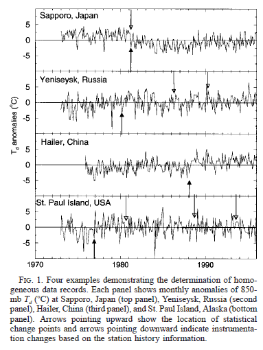
Then they have a section discussing various data homogeneity issues, which includes this graphic showing the challenge of identifying instrument changes which affect measurements:

From Ross & Elliott (2001)

From Ross & Elliott (2001)

Figure 1

They comment:

These examples show that the combination of historical and statistical information can identify some known instrument changes. However, we caution that the separation of artificial (e.g., instrument changes) and natural variability is inevitably somewhat subjective. For instance, the same instrument change at one station may not show as large an effect at another location or time of day..

Furthermore, the ability of the statistical method to detect abrupt changes depends on the variability of the record, so that the same effect of an instrument change could be obscured in a very noisy record. In this case, the same change detected at one station may not be detected at another station containing more variability.

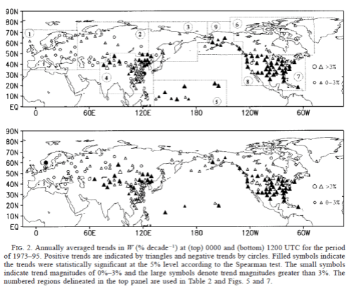
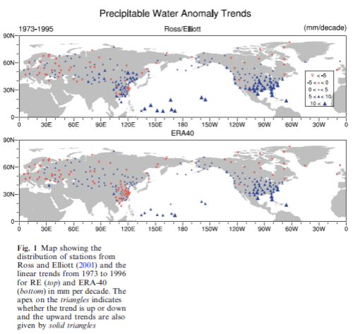
Here are their results from 1973-1995 in geographical form. Triangles are positive trends, circles are negative trends. You also get to see the distribution of radiosondes, as each marker indicates one station:

Figure 2

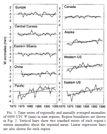
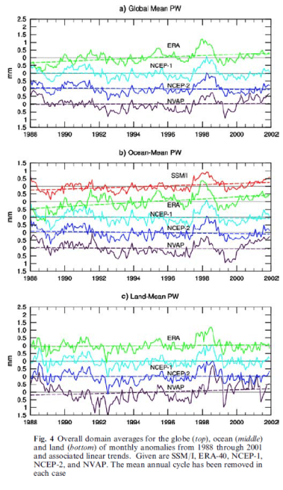
And their summary of time-based trends for each region:

Figure 3

In their summary they make some interesting comments:

We found that a global estimate could not be made because reliable records from the Southern Hemisphere were too sparse; thus we confined our analysis to the Northern Hemisphere. Even there, the analysis was limited by continual changes in instrumentation, albeit improvements, so we were left with relatively few records of total precipitable water over the era of radiosonde observations that were usable.

Emphasis added.

Well, I recommend that readers take the time to read the whole paper for themselves to understand the quality of work that has been done – and learn more about the issues with the available data.

What is Special about 1973?

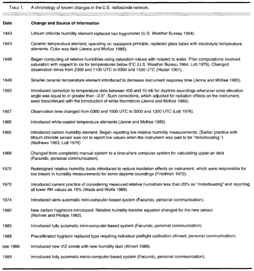
In their 1991 paper, Elliot and Gaffen showed that pre-1973 radiosonde measurements came with much more problems than post-1973.

From Elliott & Gaffen (1991)

From Elliott & Gaffen (1991)

Figure 4 – Click for larger view

Note that the above is just for the US radiosonde network.

 Our findings suggest caution is appropriate when using the humidity archives or interpreting existing water vapor climatologies so that changes in climate not be confounded by non-climate changes.

And one extract to give a flavor of the whole paper:

The introduction of the new hygristor in 1980 necessitated a new algorithm.. However, the new algorithm also eliminated the possibility of reports of humidities greater than 100% but ensured that humidities of 100% cannot be reported in cold temperatures. The overall effect of these changes is difficult to ascertain. The new algorithm should have led to higher reported humidities compared to the older algorithm, but the elimination of reports of very high values at cold temperatures would act in the opposite sense.

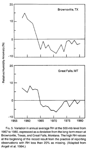
And a nice example of another change in radiosonde measurement and reporting practice. The change below is just an artifact of low humidity values being reported after a certain date:

From Elliott & Gaffen (1991)

From Elliott & Gaffen (1991)

Figure 5

As the worst cases came before 1973, most researchers subsequently reporting on water vapor trends have tended to stick to post-1973 (or report on that separately and add caveats to pre-1973 trends).

But it is important to understand that issues with radiosonde measurements are not confined to pre-1973.

Here are a few more comments, this time from Elliott in his 1995 paper:

Most (but not all) of these changes represent improvements in sensors or other practices and so are to be welcomed. Nevertheless they make it difficult to separate climate changes from changes in the measurement programs..

Since then, there have been several generations of sensors and now sensors have much faster response times. Whatever the improvements for weather forecasting, they do leave the climatologist with problems. Because relative humidity generally decreases with height slower sensors would indicate a higher humidity at a given height than today’s versions (Elliott et al., 1994).

This effect would be particularly noticeable at low temperatures where the differences in lag are greatest. A study by Soden and Lanzante (submitted) finds a moist bias in upper troposphere radiosondes using slower responding humidity sensors relative to more rapid sensors, which supports this conjecture. Such improvements would lead the unwary to conclude that some part of the atmosphere had dried over the years.

And Gaffen, Elliott & Robock (1992) reported that in analyzing data from 50 stations from 1973-1990 they found instrument changes that created “inhomogeneities in the records of about half the stations

Satellite Demonstration

Different countries tend to use different radiosondes, have different algorithms and have different reporting practices in place.

The following comparison is of upper tropospheric water vapor. As an aside this has a focus because water vapor in the upper atmosphere disproportionately affects top of atmosphere radiation – and therefore the radiation balance of the climate.

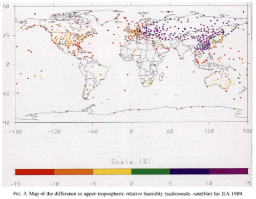
From Soden & Lanzante (1996), the data below, of the difference between satellite and radiosonde measurements, identifies a significant problem:

Soden & Lanzante (1996)

Soden & Lanzante (1996)

Figure 6

Since the same satellite is used in the comparison at all radiosonde locations, the satellite measurements serve as a fixed but not absolute reference. Thus we can infer that radiosonde values over the former Soviet Union tend to be systematically moister than the satellite measurements, that are in turn systematically moister than radiosonde values over western Europe.

However, it is not obvious from these data which of the three sets of measurements is correct in an absolute sense. That is, all three measurements could be in error with respect to the actual atmosphere..

..However, such a satellite [calibration] error would introduce a systematic bias at all locations and would not be regionally dependent like the bias shown in fig. 3 [=figure 6].

They go on to identify the radiosonde sensor used in different locations as the likely culprit. Yet, as various scientists comment in their papers, countries take on a new radiosonde in piecemeal form, sometimes having a “competitive supply” situation where 70% is from one vendor and 30% from another vendor. Other times radiosonde sensors are changed across a region over a period of a few years. Inter-comparisons are done, but inadequately.

Soden and Lanzante also comment on spatial coverage:

Over data-sparse regions such as the tropics, the limited spatial coverage can introduce systematic errors of 10-20% in terms of the relative humidity. This problem is particularly severe in the eastern tropical Pacific, which is largely void of any radiosonde stations yet is especially critical for monitoring interannual variability (e.g. ENSO).

Before we move onto reanalyses, a summing up on radiosondes from the cautious William P. Elliot (1995):

Thus there is some observational evidence for increases in moisture content in the troposphere and perhaps in the stratosphere over the last 2 decades. Because of limitations of the data sources and the relatively short record length, further observations and careful treatment of existing data will be needed to confirm a global increase.

Reanalysis – or Filling in the Blanks

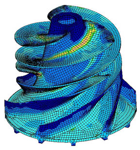
Weather forecasting and climate modelling is a form of finite element analysis (and see Wikipedia). Essentially in FEA, some kind of grid is created – like this one for a pump impellor:

Stress analysis in an impeller

Stress analysis in an impeller

Figure 7

– and the relevant equations can be solved for each boundary or each element. It’s a numerical solution to a problem that can’t be solved analytically.

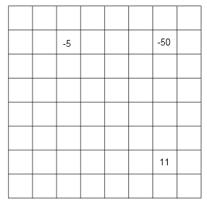
Weather forecasting and climate are as tough as they come. Anyway, the atmosphere is divided up into a grid and in each grid we need a value for temperature, pressure, humidity and many other variables.

To calculate what the weather will be like over the next week a value needs to be placed into each and every grid. And just one value. If there is no value in the grid the program can’t run and there’s nowhere to put two values.

By this massive over-simplification, hopefully you will be able to appreciate what a reanalysis does. If no data is available, it has to be created. That’s not so terrible, so long as you realize it:

Figure 8

This is a simple example where the values represent temperatures in °C as we go up through the atmosphere. The first problem is that there is a missing value. It’s not so difficult to see that some formula can be created which will give a realistic value for this missing value. Perhaps the average of all the values surrounding it? Perhaps a similar calculation which includes values further away, but with less weighting.

With some more meteorological knowledge we might develop a more sophisticated algorithm based on the expected physics.

The second problem is that we have an anomaly. Clearly the -50°C is not correct. So there needs to be an algorithm which “fixes” it. Exactly what fix to use presents the problem.

If data becomes sparser then the problems get starker. How do we fill in and correct these values?

Figure 9

It’s not at all impossible. It is done with a model. Perhaps we know surface temperature and the typical temperature profile (“lapse rate”) through the atmosphere. So the model fills in the blanks with “typical climatology” or “basic physics”.

But it is invented data. Not real data.

Even real data is subject to being changed by the model..

NCEP/NCAR Reanalysis Project

There are a number of reanalysis projects. One is the NCEP/NCAR project (NCEP = National Centers for Environmental Prediction, NCAR = National Center for Atmospheric Research).

Kalnay (1996) explains:

The basic idea of the reanalysis project is to use a frozen state-of-the-art analysis/forecast system and perform data assimilation using past data, from 1957 to the present (reanalysis).

The NCEP/NCAR 40-year reanalysis project should be a research quality dataset suitable for many uses, including weather and short-term climate research.

An important consideration is explained:

An important question that has repeatedly arisen is how to handle the inevitable changes in the observing system, especially the availability of new satellite data, which will undoubtedly have an impact on the perceived climate of the reanalysis. Basically the choices are a) to select a subset of the observations that remains stable throughout the 40-year period of the reanalysis, or b) to use all the available data at a given time.

Choice a) would lead to an reanalysis with the most stable climate, and choice b) to an analysis that is as accurate as possible throughout the 40 years. With the guidance of the advisory panel, we have chosen b), that is, to make use of the most data available at any given time.

What are the categories of output data?

  • A = analysis variable is strongly influenced by observed data and hence it is in the most reliable class
  • B = although there are observational data that directly affect the value of the variable, the model also has a very strong influence on the value
  • C = there are no observations directly affecting the variable, so that it is derived solely from the model fields

Humidity is in category B.

Interested people can read Kalnay’s paper. Reanalysis products are very handy and widely used. Those with experience usually know what they are playing around with. Newcomers need to pay attention to the warning labels.

Comparing Reanalysis of Humidity

Bengtsson et al (2004) reviewed another reanalysis project, ERA-40. They provide a good example of how incorrect trends can be introduced (especially the 2nd paragraph):

A bias changing in time can thus introduce a fictitious trend without being eliminated by the data assimilation system. A fictitious trend can be generated by the introduction of new types of observations such as from satellites and by instrumental and processing changes in general. Fictitious trends could also result from increases in observational coverage since this will affect systematic model errors.

Assume, for example, that the assimilating model has a cold bias in the upper troposphere which is a common error in many general circulation models (GCM). As the number of observations increases the weight of the model in the analysis is reduced and the bias will correspondingly become smaller. This will then result in an artificial warming trend.

Bengtsson and his colleagues analyze tropospheric temperature, IWV and kinetic energy.

ERA-40 does have a positive trend in water vapor, something we will return to. The trend from ERA-40 for 1958-2001 is +0.41 mm/decade, and for 1979-2001 = +0.36 mm/decade. They note that NCEP/NCAR has a negative trend of -0.24 mm/decade from 1958-2001 and -0.06mm/decade  for 1979-2001, but it isn’t a focus of their study.

They do an analysis which excludes satellite data and find a lower (but still positive) trend for IWV. They also question the magnitudes of tropospheric temperature trends and kinetic energy on similar grounds.

The point is essentially that the new data has created a bias in the reanalysis.

Their conclusion, following various caveats about the scale of the study so far:

Returning finally to the question in the title of this study an affirmative answer cannot be given, as the indications are that in its present form the ERA40 analyses are not suitable for long-term climate trend calculations.

However, it is believed that there are ways forward as indicated in this study which in the longer term are likely to be successful. The study also stresses the difficulties in detecting long term trends in the atmosphere and major efforts along the lines indicated here are urgently needed.

So, onto Trends and variability in column-integrated atmospheric water vapor by Trenberth, Fasullo & Smith (2005). This paper is well worth reading in full.

For years before 1996, the Ross and Elliott radiosonde dataset is used for validation of European Centre for Medium-range Weather Forecasts (ECMWF) reanalyses ERA-40. Only the special sensor microwave imager (SSM/I) dataset from remote sensing systems (RSS) has credible means, variability and trends for the oceans, but it is available only for the post-1988 period.

Major problems are found in the means, variability and trends from 1988 to 2001 for both reanalyses from National Centers for Environmental Prediction (NCEP) and the ERA-40 reanalysis over the oceans, and for the NASA water vapor project (NVAP) dataset more generally. NCEP and ERA-40 values are reasonable over land where constrained by radiosondes.

Accordingly, users of these data should take great care in accepting results as real.

Here’s a comparison of Ross & Elliott (2001) [already shown above] with ERA-40:

From Trenbert et al (2005)

From Trenberth et al (2005)

Figure 10 – Click for a larger image

Then they consider 1988-2001, the reason being that 1988 was when the SSMI (special sensor microwave imager) data over the oceans became available (more on the satellite data later).

From Trenberth et al (2005)

From Trenberth et al (2005)

Figure 11

At this point we can see that ERA-40 agrees quite well with SSMI (over the oceans, the only place where SSMI operates), but NCEP/NCAR and another reanalysis product, NVAR, produce flat trends.

Now we will take a look at a very interesting paper: The Mass of the Atmosphere: A Constraint on Global Analyses, Trenberth & Smith (2005). Most readers will probably not be aware of this comparison and so it is of “extra” interest.

The total mass of the atmosphere is in fact a fundamental quantity for all atmospheric sciences. It varies in time because of changing constituents, the most notable of which is water vapor. The total mass is directly related to surface pressure while water vapor mixing ratio is measured independently.

Accordingly, there are two sources of information on the mean annual cycle of the total mass and the associated water vapor mass. One is from measurements of surface pressure over the globe; the other is from the measurements of water vapor in the atmosphere.

The main idea is that other atmospheric mass changes have a “noise level” effect on total mass, whereas water vapor has a significant effect. As measurement of surface pressure is a fundamental meteorological value, measured around the world continuously (or, at least, continually), we can calculate the total mass of the atmosphere with high accuracy. We can also – from measurements of IWV – calculate the total mass of water vapor “independently”.

Subtracting water vapor mass from total atmospheric measured mass should give us a constant – the “dry atmospheric pressure”. That’s the idea. So if we use the surface pressure and the water vapor values from various reanalysis products we might find out some interesting bits of data..

from Trenberth & Smith (2005)

from Trenberth & Smith (2005)

Figure 12

In the top graph we see the annual cycle clearly revealed. The bottom graph is the one that should be constant for each reanalysis. This has water vapor mass removed via the values of water vapor in that reanalysis.

Pre-1973 values show up as being erratic in both NCEP and ERA-40. NCEP values show much more variability post-1979, but neither is perfect.

The focus of the paper is the mass of the atmosphere, but is still recommended reading.

Here is the geographical distribution of IWV and the differences between ERA-40 and other datasets (note that only the first graphic is trends, the following graphics are of differences between datasets):

Trenberth et al (2005)

Trenberth et al (2005)

Figure 13 – Click for a larger image

The authors comment:

The NCEP trends are more negative than others in most places, although the patterns appear related. Closer examination reveals that the main discrepancies are over the oceans. There is quite good agreement between ERA-40 and NCEP over most land areas except Africa, i.e. in areas where values are controlled by radiosondes.

There’s a lot more in the data analysis in the paper. Here are the trends from 1988 – 2001 from the various sources including ERA-40 and SSMI:

From Trenberth et al (2005)

From Trenberth et al (2005)

Figure 14 – Click for a larger view

  • SSMI has a trend of +0.37 mm/decade.
  • ERA-40  has a trend of +0.70mm/decade over the oceans.
  • NCEP has a trend of -0.1mm/decade over the oceans.

To be Continued..

As this article is already pretty long, it will be continued in Part Two, which will include Paltridge et al (2009), Dessler & Davis (2010) and some satellite measurements and papers.

Update – Part Two is published

References

On the Utility of Radiosonde Humidity Archives for Climate Studies, Elliot & Gaffen, Bulletin of the American Meteorological Society (1991)

Relationships between Tropospheric Water Vapor and Surface Temperature as Observed by Radiosondes, Gaffen, Elliott & Robock, Geophysical Research Letters (1992)

Column Water Vapor Content in Clear and Cloudy Skies, Gaffen & Elliott, Journal of Climate (1993)

On Detecting Long Term Changes in Atmospheric Moisture, Elliot, Climate Change (1995)

Tropospheric Water Vapor Climatology and Trends over North America, 1973-1993, Ross & Elliot, Journal of Climate (1996)

An assessment of satellite and radiosonde climatologies of upper-tropospheric water vapor, Soden & Lanzante, Journal of Climate (1996)

The NCEP/NCAR 40-year Reanalysis Project, Kalnay et alBulletin of the American Meteorological Society (1996)

Radiosonde-Based Northern Hemisphere Tropospheric Water Vapor Trends, Ross & Elliott, Journal of Climate (2001)

An analysis of satellite, radiosonde, and lidar observations of upper tropospheric water vapor from the Atmospheric Radiation Measurement Program, Soden et al,  Journal of Geophysical Research (2005)

The Radiative Signature of Upper Tropospheric Moistening, Soden et al, Science (2005)

The Mass of the Atmosphere: A Constraint on Global Analyses, Trenberth & Smith, Journal of Climate (2005)

Trends and variability in column-integrated atmospheric water vapor, Trenberth et al, Climate Dynamics (2005)

Can climate trends be calculated from reanalysis data? Bengtsson et al, Journal of Geophysical Research (2005)

Trends in middle- and upper-level tropospheric humidity from NCEP reanalysis data, Paltridge et al, Theoretical Applied Climatology (2009)

Trends in tropospheric humidity from reanalysis systems, Dessler & Davis, Journal of Geophysical Research (2010)

Read Full Post »