In the CO2 series we looked at the effect of CO2 without climate feedbacks. The “answer” to the doubling of CO2 was a “radiative forcing” of 3.7W/m^2 and an increase in surface temperature of about 1°C.
What about feedbacks?
There are many ways to introduce this problem. We’ll start with the great Ramanathan, who is always worth reading. This article discusses the ideas in the chapter The Radiative Forcing due to Clouds and Water Vapor (by Ramanathan and Inamdar) from Frontiers of Climate Modeling by Kiehl and Ramanathan (2006). Note that the link allows you to download the chapter. Well worth reading.
And if you have questions about whether CO2 can influence temperature or whether the inappropriately-named “greenhouse” effect exists, take a look at the CO2 series (and ask questions there).
Preamble
Various papers from the 60’s onwards that attempted to model the change in radiative flux and surface temperature (as a result of changes in CO2 concentrations) usually solved the problem using (at least) two scenarios:
- constant absolute humidity
- constant relative humidity
The reason is that absolute humidity is less realistic than relative humidity – and the concept of relative humidity leads to positive feedback. Why positive feedback? Higher concentrations of CO2 lead to increased radiative forcing and so the surface and tropospheric temperature increases. As a result – under constant relative humidity – the amount of water vapor in the troposphere increases. Water vapor is a greenhouse gas and so further increases “radiative forcing”.
One of the questions that come to people’s minds is whether this leads to thermal runaway. The answer, when considering the “extra” effect from water vapor is no, and this is because there are also negative feedbacks in the system, especially the fact that radiation (a negative feedback) increases as the 4th power of absolute temperature.
But enough of trying to think about the complete solution before we have even begun. Let’s take the time to understand the thinking behind the problem.
Cloudy Skies
Clouds are one of the toughest problems in climate science, and as a result, many models and experiments differentiate between cloudy and clear skies.
The ERBE experiments clarified the main effects from clouds.
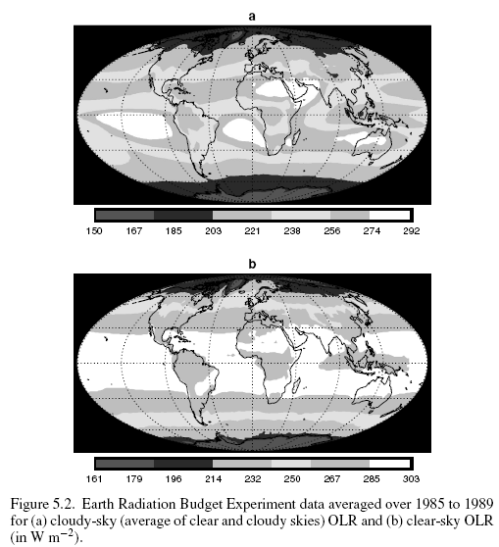
Here is OLR (outgoing longwave radiation) under clear and cloudy (=all skies) averaged over 1985-1989:
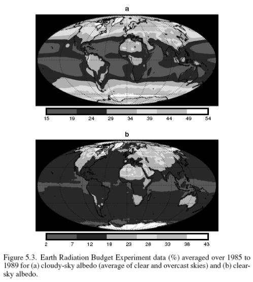
Here is the albedo (%), or % of solar radiation reflected:
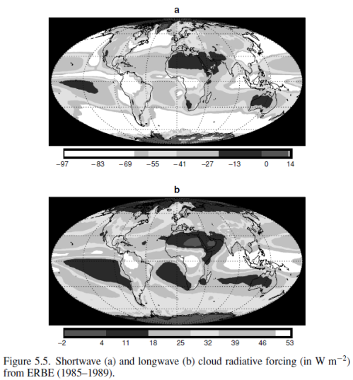
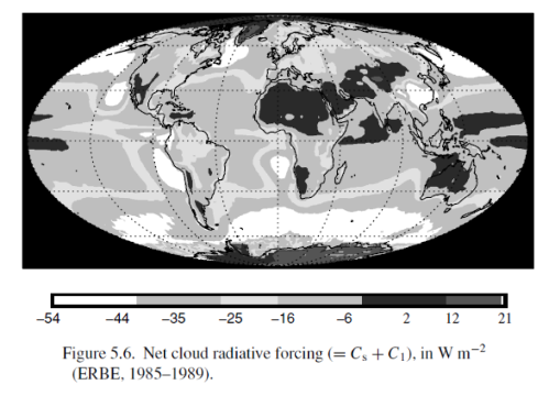
Clouds reflect solar radiation by 48 W/m2 but reduce the outgoing longwave radiation (OLR) by 30 W/m2, therefore the average net effect of clouds – over this period at least – is to cool the climate by 18 W/m2. Note that these values are the global annual average.
Here are the net shortwave (solar reflection) and net OLR effects from clouds over the whole period:
and the two effects combined:
The “Greenhouse” Effect and Water Vapor
I’ll try and keep any maths to a minimum, but a few definitions are needed.. if you don’t like seeing equations the explanations in the text mean you haven’t missed anything essential.
We will call the “greenhouse” effect of the atmosphere and clouds, G, and the average OLR (outgoing longwave radiation), F:
F = σTs4 – G
The first term on the right-hand side of the equation, σTs4, is just the radiation from the earth’s surface at a temperature of Ts (the Stefan-Boltzmann equation). So the radiation from the earth’s surface less the “greenhouse” effect is the amount of radiation that escapes to space.
G is made up of the clear sky “greenhouse” effect, Gclear, and the (longwave) effect of clouds, Gcloud.
Now as we move from the hotter equator to the colder poles we would expect Gclear to reduce simply because the surface radiation is much reduced – a 30°C surface emits 480 W/m2 and a 0°C surface emits 315 W/m2. A large proportion of the changes in the “greenhouse” effect, Gclear, are simply due to changes in surface temperature.
Therefore, we introduce a normalized “greenhouse” effect, gclear:
gclear = Gclear / σTs4
This parameter simply expresses the ratio between the clear sky “greenhouse” effect and the surface radiation. The variations in this normalized value reflect changes in atmospheric humidity and lapse rates (the temperature profile up through the atmosphere). See especially CO2 – An Insignificant Trace Gas? Part Five for a little more illumination on this.
The global average value for Gclear = 131 W/m2 and for gclear = 0.33 – i.e., the atmosphere reduces the radiation escaping to space by 33%.
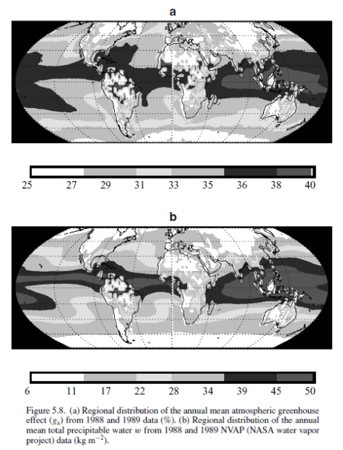
Here is how gclear varies around the world (top graphic) compared with water vapor around the world (bottom graphic):
It should be clear from these graphics that observed variations in the normalized “greenhouse” effect are largely due to changes in water vapor. [Note – change of notation from the graphics – ga in the graphic is gclear in my text]
Water vapor decreases from equator to pole due to temperature (lower temperatures mean lower absolute humidity), and increases over ocean compared with land (because of the availability of water to evaporate).
Feedback
If we can see that the “greenhouse” effect is strongly influenced by water vapor, we want to know how water vapor changes in response to surface and tropospheric temperature changes.
To make sense of this section it’s helpful to follow some maths. However, I recognize that many people would rather skip any maths so this is in the last section for reference.
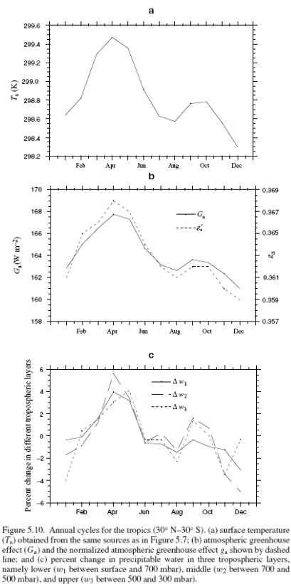
Here are the results from ERBE for: the tropics (30°N – 30°S) with surface temperature; the “greenhouse” effect + the normalized version; and the change in water vapor in different vertical sections of the atmosphere:
Ramanathan says:
For the tropics, Ts peaks in March/April, while for 90°N–90°S, Ts peaks in July. We can qualitatively interpret the phase of the annual cycle as follows. The tropical annual cycle is dominated by the coupled ocean–atmosphere system and as a result, the temperature response lags behind the forcing by a maximum of about three months (π/2); thus, with the solar insolation peaking in December 21, the temperature peaks in late March as shown in Figure 10.
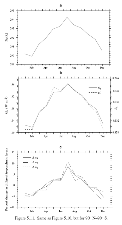
Now the whole globe as a comparison:
Ramanathan again:
The extra-tropical and global annual cycle is most likely dominated by the hemispherical asymmetry in the land fraction. During the northern-hemisphere summer (June, July, and August), the large land masses warm rapidly (with about a one month lag) which dominates the hemispherical and global mean response; however, during the southern-hemisphere summer, the relatively smaller fraction of land prevents a corresponding response. Thus, the globe is warmest during June/July and is coldest during December/January.
What can we make of the correlation? Correlation doesn’t equal causation.
The best fit is a phase lag of less than a month which implies that water vapor and gclear are not driving Ts – because the feedback in that case would require more than one month. The converse, that Ts is driving water vapor and gclear, is much more likely because convective time scales are very short.
Of course, this is a deduction from a limited time period.
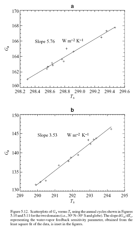
One of the key relationships in understanding feedback is the change in Gclear with Ts (mathematically we write this as dGclear/dTs – which means “the rate of change with Gclear as Ts varies “).
For reasons briefly outlined in the maths section, if dGclear / dTs > 2.2 it implies positive feedback from the climate.
When the data is plotted from the ERBE data we can see that in the tropics the value is the highest, much greater than 2.2, and when the whole globe is included the value reduces significantly. However, the value for the whole globe still implies positive feedback.
In this last graph we see the feedback value for progressively wider latitude ranges – so on the left we are only looking at the tropics, while over on the right (90°N to 90°S) we are looking at the entire planet. This helps to see the contribution from the tropics progressively outweighed by the rest of the plant – so the important point is that without the strong effect from the tropics the feedback might well have moved to negative.
The feedback doesn’t change between clear sky and all sky, implying that the cloud feedback doesn’t impact the climate system feedback (on these timescales).
Ramanathan comments:
However, our results do not necessarily confirm the positive feedback resulting from the fixed relative humidity models for global warming, for the present results are based on annual cycle. We need additional tests with decadal time-scale data for a rigorous test. Nevertheless, the analysis confirms that water vapor has a positive feedback effect for global-scale changes on seasonal to inter-annual time scales.
He also comments on other work (including Lindzen) that finds different results for the relative important of water vapor in different vertical sections of the troposphere.
Hopefully, we will get the opportunity to consider these in future articles.
Articles in this Series
Part One – Responses – answering some questions about Part One
Part Two – some introductory ideas about water vapor including measurements
Part Three – effects of water vapor at different heights (non-linearity issues), problems of the 3d motion of air in the water vapor problem and some calculations over a few decades
Part Four – discussion and results of a paper by Dessler et al using the latest AIRS and CERES data to calculate current atmospheric and water vapor feedback vs height and surface temperature
Part Five – Back of the envelope calcs from Pierrehumbert – focusing on a 1995 paper by Pierrehumbert to show some basics about circulation within the tropics and how the drier subsiding regions of the circulation contribute to cooling the tropics
Part Six – Nonlinearity and Dry Atmospheres – demonstrating that different distributions of water vapor yet with the same mean can result in different radiation to space, and how this is important for drier regions like the sub-tropics
Part Seven – Upper Tropospheric Models & Measurement – recent measurements from AIRS showing upper tropospheric water vapor increases with surface temperature
Conclusion
This is a big subject which has lots of different perspectives, and only one is developed here. Therefore, I hope that this is the first of many articles on the subject.
It should be helpful to see the approach and one way of interpreting the data. There is a theoretical framework behind the concepts, which can be seen in Ramanathan’s paper from 1981: The Role of Ocean-Atmosphere Interaction in the CO2 Climate Problem. (You can find a free copy online). It’s quite involved but perhaps some of the concepts from this paper will be in one of the next posts in this series.
Maths
I’ll follow the notations from the chapter reasonably closely. But I think they are confusing so I have changed a few of them.
And if you do want to understand the maths it’s definitely worth taking a look at the more detailed explanations in the chapter to understand this beyond the surface.
F = OLR (outgoing longwave radiation)
F = Fclear (1-f) + f.Fcloudy, where f is the fraction of clouds, and Fclear is the clear sky OLR
F = σTs4 – G [1], where G is the “greenhouse” effect
and G = Gclear + Gcloud [2]
Now the main feedback parameter is dF/dTs, so:
dF/dTs = 4σTs3 – dG/dTs = 4σTs3 – (dGclear/dTs + dGcloud/dTs) [3]
Note that 4σTs3 = 5.5 Wm-2K-1 (at T=289K)
Background: dGclear/dTs is affected by water vapor and lapse rate and dGcloud/dTs is affected by cloud feedback and lapse rate
Now dGclear/dTs = 4σTs3 – dFclear/dTs [4]
now for Ts changing with no lapse rate feedback and no water vapor feedback, dFclear/dTs = 3.3 Wm-2K-1 (from Ramanathan 1981, see ref above in conclusion).
Therefore, if there is positive feedback dFclear/dTs < 3.3 Wm-2K-1 and if negative feedback dFclear/dTs > 3.3 Wm-2K-1 – because a lower value of F (OLR) means a higher value of G (greenhouse effect)
And from [4], if dGclear/dTs > 5.5 – 3.3 = 2.2 then there is positive feedback.



The Woody Guthrie award
Posted in Commentary on May 19, 2010| 16 Comments »
This is a very quick post to say thanks to John Cook of Skeptical Science for the recent “Woody Guthrie award for a thinking blogger” and especially the kind comments he made.
I’m proud to be the recipient and already in a panic about the next recipient, apparently it’s up to me to decide. It is especially a problem in this divided world we live in.
I’m very happy that many sides of the climate debate visit this blog and contribute and ask questions. I can only ask again what I ask in About This Blog:
Read Full Post »