Once we start measuring climate parameters we get a lot of data. To compare datasets, or datasets with models, we can look at means, standard deviations, medians, percentiles, and so on.
I’ve frequently mentioned the problem that climate is nonlinear. If we investigate the underlying physics of most processes we find that the answer to the problem does not scale linearly as inputs change.
Roca et al (2012) say:
The main reason for water vapor to be of importance to the energetics of the climate lies in the nonlinearity of the radiative transfer to the humidity. The outgoing longwave radiation (OLR) is indeed much more sensitive to a given perturbation in a dry rather than moist environment, conferring a central role of the moisture distribution in these regions to the radiation budget of the planet and to the overall climate sensitivity.
The authors demonstrate that with the same mean value of water vapor in a dry climate we can get different values of radiation to space for different distributions. (Note that FTH = free tropospheric humidity. This is the humidity above the atmospheric boundary layer – the boundary layer ranges from between a few hundred meters and one km):
Energy constraints on planet Earth (i.e. applying the first law of thermodynamics) require that, at equilibrium, the Earth emits in the long wave as much radiation as its gets from the Sun. This budget approach is hence focused on the mean values of the OLR over the whole planet and over long time scales corresponding to the global radiative-convective equilibrium theory.
While the mean OLR is the constrained parameter, owing to the nonlinearity of the clear-sky radiative transfer to water vapour (Figs. 2a, 3), the whole distribution of moisture has to be considered rather than its mean in order to link the distribution of humidity to that of radiation.
To illustrate this, the OLR sensitivity to FTH curve (Fig. 2a) and four distributions of FTH for a dry case are considered (Fig. 2bc): a constant distribution with mean of 14.5%, an uniform distribution with mean of 14.5% bounded within plus or minus 5%, a Gaussian distribution with mean of 14.5% (and a 5% standard deviation) and a generalized log-normal distribution with a mean of 14.5% shown in Fig. 2c. The mean OLR corresponding to the constant distribution is 311 W/m². The uniform and normal distribution yield to a mean OLR larger by 0.7 W/m² in both cases.
The log-normal PDF, on the other hand, gives a 3 W/m² overestimation of the OLR with respect to the constant case. At the scale of the doubling of CO2 problem, such a systematic bias could be significant depending on its geographical spread, which is explored next.
PDF is the probability density function.
And in case it’s not clear what the authors were saying, the same average humidity can result in significantly different OLR depending on the distribution of the humidity from which the average was calculated.
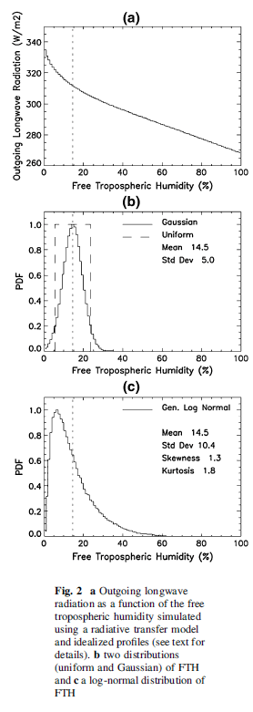
Figure 1
We saw the importance of the drier subsiding regions of the tropics in Clouds & Water Vapor – Part Five – Back of the envelope calcs from Pierrehumbert in that they have much higher OLR than the convective regions.
This paper calculates the results (using the vertical profile of temperature as a multi-year summer average of Bay of Bengal conditions from ERA-40) that with a constant boundary layer humidity (BLH), increasing FTH from 1% to 15% reduces OLR by 23 W/m². Increasing FTH from 35% to 50% reduces OLR by only 8 W/m². The spectral composition of these changes is interesting:
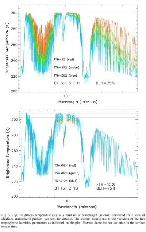
Figure 2
The authors comment that the changes in surface temperature (in the 2nd graph) result in a smaller change in OLR, which seems to be indicated from the brightness temperature graph. I have asked Remy Roca if he has the OLR calculations for this second graph to hand.
Then a statistical test is applied to values of humidity at 500 hPa (about 5.5 km altitude):

Figure 3
We see that the moist areas are more likely to have a normal (gaussian) distribution, while the dry areas are less likely.
Here is an actual distribution from Ryoo et al (2008), for different regions from 250 hPa (about 11km) for both tropical (red) and sub-tropical regions (blue):
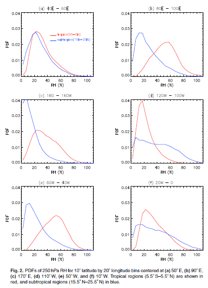
Figure 4
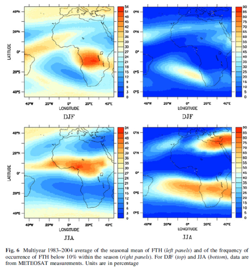
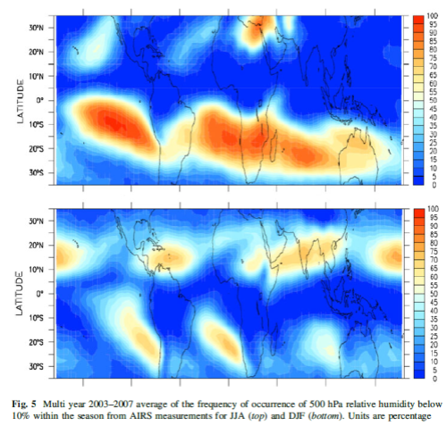
The authors use the frequency of occurrence of relative humidity less than 10% as a measure:
The need of handling the whole PDF of humidity instead of only the mean of the field implies the manipulation of the upper moments of the distribution (skewness and kurtosis). While the computations are straightforward, the comparison of two PDFs through the comparison of their 4 moments is not. Assuming a generalized log-normal distribution also requires 4 parameters to be fitted. It can be brought down to 2 parameters by imposing the lower and upper range limit of the distribution (0 and 100% for instance) at the cost of limiting the possible distributions.
The simplified model (Ryoo et al. 2009) also comprises only two parameters, linked to the first two moments of the distribution. Still, the moments-to-moments comparison of PDFs remains difficult.
Here, it is proposed to limit the analysis to a single parameter characterizing the PDF with emphasis on the dry foot of the distribution: the frequency of occurrence of RH below 10%, noted in the following as RHp10.
The paper then provides some graphs of the frequency of RH below 10%. We can think of it as another way of looking at the same data, but focusing on the drier end of the dataset:
From Roca et al 2012
Figure 5
From Roca et al 2012
Figure 6
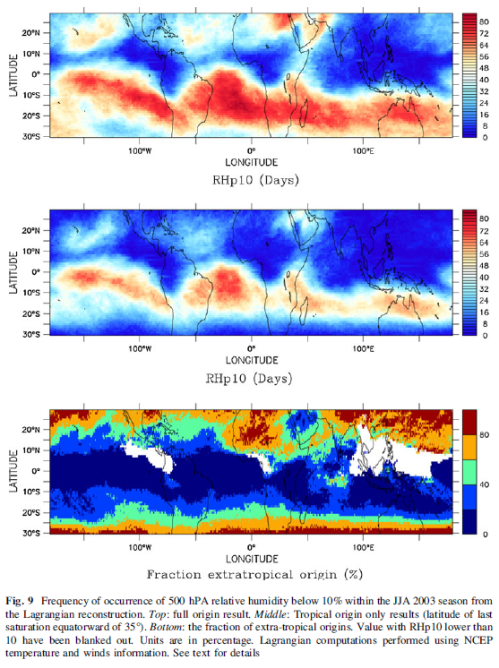
The authors then consider the source of the driest air at 500hPa. Now this uses what is called the advection-condensation method, something I hope to cover in a later article on water vapor. But for interest, here is their result:
From Roca et al 2012
Figure 7
The middle graph is the first graph with air sourced from the extra-tropics excluded.
The RHp10 distribution of the reconstructed field for the boreal summer 2003 is compared to the RHp10 distribution obtained by keeping only the air masses that experienced last saturation within the intertropical belt (35S–35N) in Fig. 9. Excluding the extra-tropical last saturated air masses overall moistens the atmosphere. The domain averaged RHp10 decreases from 37 to 23% without the extra-tropical influence. While the patterns overall remain similar within the two computations, the driest areas nevertheless appear more impacted and less spread in the tropics only case (Fig. 9 middle). The very dry features in the subtropical south Atlantic is mainly built from tropical originating air with the fraction of extra-tropical influence less than 10% (Fig. 9c).
Conclusion
Even if a monthly mean value of a climatological value from a model matches the measurement monthly mean it doesn’t necessarily mean that the consequences for the climate are the same.
Small changes in the distribution of values (for the same average) can have significant impacts. Here we see that this is the case for dry regions.
In Clouds & Water Vapor – Part Five – Back of the envelope calcs from Pierrehumbert we saw that these dry regions have a big role in cooling the tropics and therefore in regulating the temperature of the planet. Understanding more about the distribution of humidity and the mechanisms and causes is essential for progress in climate science.
Articles in the Series
Part One – introducing some ideas from Ramanathan from ERBE 1985 – 1989 results
Part One – Responses – answering some questions about Part One
Part Two – some introductory ideas about water vapor including measurements
Part Three – effects of water vapor at different heights (non-linearity issues), problems of the 3d motion of air in the water vapor problem and some calculations over a few decades
Part Four – discussion and results of a paper by Dessler et al using the latest AIRS and CERES data to calculate current atmospheric and water vapor feedback vs height and surface temperature
Part Five – Back of the envelope calcs from Pierrehumbert – focusing on a 1995 paper by Pierrehumbert to show some basics about circulation within the tropics and how the drier subsiding regions of the circulation contribute to cooling the tropics
Part Six – Nonlinearity and Dry Atmospheres – demonstrating that different distributions of water vapor yet with the same mean can result in different radiation to space, and how this is important for drier regions like the sub-tropics
Part Seven – Upper Tropospheric Models & Measurement – recent measurements from AIRS showing upper tropospheric water vapor increases with surface temperature
Part Eight – Clear Sky Comparison of Models with ERBE and CERES – a paper from Chung et al (2010) showing clear sky OLR vs temperature vs models for a number of cases
Part Nine – Data I – Ts vs OLR – data from CERES on OLR compared with surface temperature from NCAR – and what we determine
Part Ten – Data II – Ts vs OLR – more on the data
References
Tropical and Extra-Tropical Influences on the Distribution of Free Tropospheric Humidity over the Intertropical Belt, Roca et al, Surveys in Geophysics (2012) – paywall paper
Variability of subtropical upper tropospheric humidity, Ryoo, Waugh & Gettelman, Atmospheric Chemistry and Physics Discussions (2008) – free paper


SoD,
That issue of Surveys in Geophysics with the article of Roca et al seems to contain many other interesting articles as well by authors like Lyman, Palmer, Trenberth and others. Have you looked at many of them?
Pekka,
I can’t recall how I came across the Roca paper in the first place. It turns out I had looked at one other paper in that issue, not sure whether by chance.
Since you commented I have looked at a number of them, mostly very interesting.
For others, here are the titles and authors of the articles:
In this issue (28 articles)
Foreword: International Space Science Institute (ISSI) Workshop on Observing and Modeling Earth’s Energy Flows
Lennart Bengtsson Pages 333-336
Understanding and Measuring Earth’s Energy Budget: From Fourier, Humboldt, and Tyndall to CERES and Beyond
Robert Kandel Pages 337-350
Climate and Earth’s Energy Flows
Matthew D. Palmer Pages 351-357
Advances in Understanding Top-of-Atmosphere Radiation Variability from Satellite Observations
Norman G. Loeb, Seiji Kato, Wenying Su, Takmeng Wong, Fred G. Rose… Pages 359-385
Estimating Global Energy Flow from the Global Upper Ocean
John M. Lyman Pages 387-393
Uncertainty Estimate of Surface Irradiances Computed with MODIS-, CALIPSO-, and CloudSat-Derived Cloud and Aerosol Properties
Seiji Kato, Norman G. Loeb, David A. Rutan, Fred G. Rose… Pages 395-412
Tracking Earth’s Energy: From El Niño to Global Warming
Kevin E. Trenberth, John T. Fasullo Pages 413-426
Changes in Earth’s Energy Flows and Clouds in 228-Year Simulation with a High-Resolution AGCM
Masato Sugi Pages 427-443
Solar Forcing of Climate
C. de Jager Pages 445-451
Total Solar Irradiance Observations
Claus Fröhlich Pages 453-473
Solar Irradiance Models and Measurements: A Comparison in the 220–240 nm wavelength band
Yvonne C. Unruh, Will T. Ball, Natalie A. Krivova Pages 475-481
Influence of the Precipitating Energetic Particles on Atmospheric Chemistry and Climate
E. Rozanov, M. Calisto, T. Egorova, T. Peter, W. Schmutz Pages 483-501
Solar Influence on Global and Regional Climates
Mike Lockwood Pages 503-534
The Water Vapour Continuum: Brief History and Recent Developments
Keith P. Shine, Igor V. Ptashnik, Gaby Rädel Pages 535-555
The Role of Water Vapour in Earth’s Energy Flows
Richard P. Allan Pages 557-564
Tropical and Extra-Tropical Influences on the Distribution of Free Tropospheric Humidity Over the Intertropical Belt
Rémy Roca, Rodrigo Guzman, Julien Lemond, Joke Meijer… Pages 565-583
Energetic Constraints on Precipitation Under Climate Change
Paul A. O’Gorman, Richard P. Allan, Michael P. Byrne… Pages 585-608
The Role of Clouds: An Introduction and Rapporteur Report
Patrick C. Taylor Pages 609-617
Cloud Adjustment and its Role in CO2 Radiative Forcing and Climate Sensitivity: A Review
Timothy Andrews, Jonathan M. Gregory, Piers M. Forster… Pages 619-635
Representing the Sensitivity of Convective Cloud Systems to Tropospheric Humidity in General Circulation Models
Anthony D. Del Genio Pages 637-656
Computation of Solar Radiative Fluxes by 1D and 3D Methods Using Cloudy Atmospheres Inferred from A-train Satellite Data
H. W. Barker, S. Kato, T. Wehr Pages 657-676
The Clouds of the Middle Troposphere: Composition, Radiative Impact, and Global Distribution
Kenneth Sassen, Zhien Wang Pages 677-691
Aerosol Forcing: Rapporteur’s Report and Summary
Frida A-M. Bender Pages 693-700
Reducing the Uncertainties in Direct Aerosol Radiative Forcing
Ralph A. Kahn Pages 701-721
Greenhouse Gases, Aerosols and Reducing Future Climate Uncertainties
Hervé Le Treut Pages 723-731
Diagnosing Climate Feedbacks in Coupled Ocean–Atmosphere Models
Eui-Seok Chung, Brian J. Soden, Amy C. Clement Pages 733-744
Determination of Earth’s Transient and Equilibrium Climate Sensitivities from Observations Over the Twentieth Century: Strong Dependence on Assumed Forcing
Stephen E. Schwartz Pages 745-777
Observing and Modeling Earth’s Energy Flows
Bjorn Stevens, Stephen E. Schwartz Pages 779-816
I’m sure no one from Surveys in Geophysics will mind me quoting the forward in full:
The Earth’s climate, as well as planetary climates in general, is broadly regulated by three fundamental parameters: the total solar irradiance, the planetary albedo and the planetary emissivity. Observations from series of different satellites during the last three decades indicate that these three quantities are generally very stable.
The total solar irradiation of some 1,361 W/m2 at 1 A.U. varies within 1 W/m2 during the 11-year solar cycle (Fröhlich 2012). The albedo is close to 29 % with minute changes from year to year but with marked zonal differences (Stevens and Schwartz 2012). The only exception to the overall stability is a minor decrease in the planetary emissivity (the ratio between the radiation to space and the radiation from the surface of the Earth). This is a consequence of the increase in atmospheric greenhouse gas amounts making the atmosphere gradually more opaque to long-wave terrestrial radiation. As a consequence, radiation processes are slightly out of balance as less heat is leaving the Earth in the form of thermal radiation than the amount of heat from the incoming solar radiation.
Present space-based systems cannot yet measure this imbalance, but the effect can be inferred from the increase in heat in the oceans where most of the heat accumulates. Minor amounts of heat are used to melt ice and to warm the atmosphere and the surface of the Earth.
The reverse is happening when there is a volcanic eruption that emits particles that reflect solar radiation. In this case less heat is entering the Earth’s system than leaving it and a cooling take place, as the system is moving toward another equilibrium.
In reality the Earth’s system is never in equilibrium as it is continuously exposed to disturbances in its energy balance. In addition to external and anthropogenic effects there are natural processes in the Earth’s system caused by variations in the cloud cover, in the exchange of heat between ocean and atmosphere, in the surface conditions such as snow and ice cover, and in changes in the three-dimensional distribution of water vapor. Other changes in the energy balance include land vegetation that affects both the surface albedo and the surface fluxes of heat and water.
Some of the processes now affecting the Earth’s climate system are relatively well understood, and others less so.
The radiative effect of the greenhouse gases added to the atmosphere since the beginning of the industrialization at the end of the eighteenth century is equivalent to a reduction in the outgoing radiation to space by some 2.8 W/m2. Less well understood are the radiative effects of anthropogenic aerosols, but an overall cooling effect of the order of 1 W/m2 is suggested. The Earth has partly adjusted to this by increasing its surface temperature by 0.6–0.8 °C during the same period, but the radiation balance has not yet been restored. Based on the ongoing warming of the oceans the radiation imbalance during the last decades is estimated to be of the order of 0.5 W/m2 with generally higher values in later years.
Other associated changes of importance for the Earth’s climate follow a temperature increase, including an increasing amount of water vapor in the atmosphere. The water vapor amount adjusts rapidly to atmospheric temperature by about 6–7 % for each degree of warming.
The scientific papers in the present volume address different observational and modeling aspects of the Earth’s energy flows. It represents the outcome of the second workshop held within the ISSI Earth Science Programme The workshop took place from 10 to 14 January, 2011, in Bern, Switzerland, with the objective of providing an in-depth overview of the Earth’s energy flows.
The participants in the workshop were experts in a wide range of disciplines and included solar physicists, experts on space observations, atmospheric radiation experts, meteorologists, oceanographers and climate modelers.
While the radiative forcing of the Earth has undergone many changes over time with consequences for the climate, the scientific interest and public concern during the last few decades have been focused on anthropogenic changes of the composition of the atmosphere and its effects on the climate.
During the last 50 years, CO2 amounts have increased by 75 ppm or by almost 25 %. The amounts of other important greenhouse gases, CH4, N2O and the CFCs, have also increased significantly. Such rapid increases were not previously encountered during the long history of our planet. During the same time, anthropogenic aerosols have also increased and affected the radiation balance by offsetting part of the greenhouse warming.
The ability of the greenhouse gases including water vapor to absorb long-wave radiation, such as the heat radiation from the Earth, has been known since the nineteenth century as described in the presentation by Kandel (2012). The main effect of the greenhouse gases is to warm the lower atmosphere, the troposphere, and to cool the lower stratosphere. Such a warming signature is presently observed, suggesting that the increasing amounts of greenhouse gases are the main cause of the observed global warming. A corresponding contribution by solar radiation would have had a different signature, as the warming in this case would encompass the full depth of the atmosphere. Furthermore, as documented in this issue, the best estimate of surface and lower tropospheric temperature suggests that the solar influence is small compared to the anthropogenic forcing. It appears that the modulation of low altitude clouds by galactic cosmic rays is unlikely to provide an explanation to the observed temperature increase (Lockwood 2012).
Three central issues were at the forefront of the Workshop:
Firstly, how accurately can we estimate the present forcing of the Earth’s system?
Secondly, how well do we know the flow of energy in the Earth’s system?
Thirdly, how well can we determine the response to the forcing, including the internal energy feedbacks of the Earth’s system?
The external radiative forcing of the system is the solar irradiation and its variation, anthropogenic greenhouse gases and aerosols, plus aerosols from volcanic eruptions.
We know that the Earth presently is receiving more heat than it emits, although present observations cannot yet measure this imbalance. However, as is shown in some of the papers in this issue, the imbalance can be estimated from the accumulation of heat in the Earth’s system where some 90 % ends up in the oceans. For the period 1993–2008 Lyman (2012) has estimated the heat flux in the upper 700 m of the ocean, normalized for the full area of the Earth, to be 0.64 ± 0.11 W/m2. For shorter periods, variations in the trends are considerable, suggesting that the irregular warming of the lower atmosphere and the surface of the Earth is probably related to the irregular warming of the deeper parts of the ocean (Trenberth and Fasullo 2012).
The energy flow within the atmosphere and between the ocean, land and atmosphere and the energy fluxes in global and annual average are known to within 1–2 W/m2 but with slightly larger values (say ±5 W/m2) for the atmospheric absorption of solar radiation and the down-welling long-wave radiation at the surface. The workshop identified the need to determine these factors more accurately.
Perhaps, the most difficult problem is to estimate or calculate the climate response to forcing perturbations; most of the presentations and discussions at the workshop were concerned with exploring a multitude of issues in this context that need to be better understood.
The direct effect of increasing the amounts of greenhouse gases in equilibrium is straightforward to calculate as it can in principle be obtained from the Stefan–Boltzmann equation. That readily shows that a relative change in radiative forcing, dF, is related to temperature change, dT, as dF/F = 4dT/T, where the forcing is measured in W/m2 and the temperature in degrees Kelvin. A doubling of CO2 is equivalent to ~3.7 W/m2 which means that the corresponding increase in temperature, dT, is about 1.1 K. This is the increased equilibrium temperature that the system will gradually approach.
What significantly complicate the situation are the feedback processes of the Earth’s system that will either decrease or increase this value. Atmospheric water vapor follows temperature and will act as a positive feedback factor as water vapor in itself is a powerful greenhouse gas. Surface albedo is also likely to exercise a positive feedback as melting ice and snow at higher temperatures are likely to lead to reduced reflectivity of solar radiation.
However, the largest problem is related to clouds. Clouds reflect solar radiation and consequently cool the Earth’s system, but clouds also enhance the absorption of terrestrial radiation. The reflected amount dominates, so the combined effect indicates a net cooling by some 20 W/m2. Of particular importance here are stratiform clouds over the oceans at low latitudes where they act as powerful regulators of the global temperature. Any changes in the amount of clouds in these areas will have a major influence on how the global temperature will evolve. The reason for this is the large difference in albedo of these clouds compared to the underlying ocean.
The possible cloud feedback, that is how a warmer climate in turn will affect the clouds, is poorly understood. It is also the main reason that climate models such as those used within the Intergovernmental Panel for Climate Change (IPCC) provide such widely different results.
The reason for the comparatively slow and irregular warming of the Earth’s system during the last century is still in many respects an open scientific issue.
A possible explanation by Schwartz (2012) is the different response timescales between the atmosphere and upper ocean areas, on the one hand, and the deep ocean, on the other hand. The upper layers determine what we might call transient climate sensitivity while the deep ocean determines the equilibrium response. The timescales of the two compartments differ widely, from the order of a decade for the upper ocean layer to several 100 years when we include the lower ocean compartment. Schwartz’s results suggest that transient processes with a modest warming might be more representative of the present century while the planet over longer times will gradually approach a higher surface temperature as it moves toward radiation equilibrium.
The present issue includes the majority of papers presented at the workshop and includes a summary of each of the different subsections. In spite of impressive scientific progress in recent years, the need for continuous space observations must be highlighted. Firstly, because of the complexity of the Earth’s energy flows including their high variability in time and space (mainly because of clouds), that will require a comprehensive sampling that must satisfactorily cover the diurnal cycle in different parts of the world. Secondly, a long-term commitment to Earth’s radiation measurements is essential because of low-frequency variations caused by both external (solar and volcanic) and anthropogenic effects, as well by different internal variations of the climate system.
SoD,
That foreword by Lennart Bengtsson is open access and so are eleven other articles from that issue
http://link.springer.com/journal/10712/33/3/page/1
At least my browser shows a lock on articles that are not open access and no lock on the open access ones.
The open access articles include that by Trenberth and Fasullo as well as the paper of Stevens and Schwartz.
Springer charges $3000 from the author (institute) to allow open access.
SOD, the summary mentions that
“The water vapor amount adjusts rapidly to atmospheric temperature by about 6–7 % for each degree of warming.”
I have often wondered about this statement. Does it take into account that the warming has not been uniform across the globe? Since more warming has occurred in the colder climates, it seems to me that the increase in total water vapor would be less. For example, at a RH of 60%, the total water vapor is about 2.5g/kg of air at 0C, but it is about 16g/kg at 30C according to the chart at the following link.
http://www.ohio.edu/mechanical/thermo/Applied/Chapt.7_11/Chapter10b.html
So a 2 degree increase in an initial 0C parcel of air and a 0 degree increase from a 30C parcel of air would result in less total water vapor increase than a 1 Degree increase in an initial 0C parcel of air and a 1 degree increase in an initial 30C parcel of air as can be easily seen looking at the curve in the above link. Of course that assumes constant RH.
Disclosure – I’m not at the same level of knowledge and expertise as most of the commenters on your site.
The value 6-7% is probably from the (paywalled) article of Allan in the same issue. There Allan writes:
The O’Gorman and Muller paper is open access. The paper is based on model simulation and does the into account regional factors. Its abstract tells
John,
This plot may be of help:
The ‘water column’ is the water vapor amount (or H2O density) in the atmosphere. The data unambiguously confirms that warmer temperatures result in increased water vapor in the air as frequently claimed. It does show the rate of increase per degree is less the colder it is and more the warmer it is. Is this what you mean?
You can clearly see that at and above the current global average temperature (about 287K), the rate of increase in water vapor is quite high per degree of warming.
John,
You do bring up and interesting point in that the planet as a whole doesn’t necessarily warm uniformaly. I think most of the warming is supposed to occur in the higher latitudes.
Thanks Pekka & RW
But why is the net effect of clouds to cool by about 20 W/m^2 in the current climate?
RW,
This was answered in Clouds & Water Vapor – Part One:
Yeah, I know about that. I meant the physical reason why.
As best I know, no one has proposed an answer and really doesn’t know. Please correct me if I’m wrong on this.
This would seem to be the 64 million dollar question that no one knows the answer to (except of course, GW).
At any rate, I think this graph provides not only the answer to why the net effect of clouds is to cool by about 20 W/m^2, but also provides the answer to the critical cloud feedback question:
It’s a scatter plot of 25 years of satellite measurements from ISCCP (1983-2008). The green and blue dots are the averages for each 2.5 degree slice of latitude in each hemisphere. Each small orange dot represents a monthly average for one sampled grid area in a 2.5 degree slice of latitude. There are more individual grid areas in the tropics compared to the areas closer to the poles, because the total area from east to west decreases with latitude.
What makes this plot and data unique is it’s just the total cloud amount independent of cloud type or combination of cloud types. The inflection point around 0C is where the net effect of increasing/decreasing clouds switches from warming to cooling. The net effect at and above the current global average temperature is unambiguously to cool.
I think we can all agree that understanding why the net effect currently is to cool would be important if one is trying to figure out what the net effect will be on incremental warming, right? I hope so.
My understanding of this is as follows:
The x axis is the surface temperature in degrees K and the y axis is the cloud covered percentage of each individual sample taken (the orange dots). For example, if the y axis is 0.6, this means that 60% of the sampled section was cloud covered and 40% was cloudless or clear sky. The ‘surface temperature’ is literally just the actual surface temperature at the time of each sample section (i.e. each grid area measured). The ‘freezing point’ reference (if it isn’t obvious) is just 273K (0C).
Do you see how at temperatures above about 0C the net effect of clouds on average is to cool, and below 0C the net effect of clouds is to warm? That is above 0C, the more clouds there happen to be the cooler it is on average, and below 0C, the more clouds there are the warmer it is on average?
Do you agree that ice and snow are roughly as reflective to solar energy as clouds are? Do you agree that ice and snow generally only persists at temperatures at or below 0C? Do you agree that on global average, most of the Earth is not snow and/or ice covered? Is it just a coincidence that the net effect of clouds switches from warming to cooling at about the same point that the surface becomes less reflective than the clouds above?
Can you see the fundamental physical mechanism behind this? Above 0C, clouds are more reflective than the surface, so the net effect of clouds is to cool by reflecting more incoming solar energy away than is delayed beneath them (i.e. re-directed back toward the surface). Below 0C, clouds are about equally reflective to solar energy as the surface is (due to snow and ice), so the net effect of clouds is to warm by delaying more energy beneath them than is reflected away in total. Clouds on average are much more opaque to outgoing infrared radiation emitted from the surface than the clear sky is.
In a warming world, if anything, less of the surface would be snow and ice covered (not more). Hardly a case for the net effect of clouds acting to warm instead of cool on incremental global warming.
Honestly, I’ve never seen anyone come up with a better explanation than this. If someone has what the they think is better explanation, I’d love to hear it.
Another way of explaining this which may be easier to see and understand is as clouds increase at temperatures above about 0C, on average the surface temperature cools and as clouds decrease the surface temperature warms. At temperatures below about 0C on the other hand, as clouds increase, the surface temperature warms and as clouds decrease the surface temperature cools. The signature of this in the data itself is independent of why the clouds increase or decrease, though if you can grasp the somewhat counterintuitive nature of how feedback works, the direction of causation is that above 0C increasing cloud coverage causes cooling and decreasing cloud coverage causes warming.
If this is hard to see or grasp, take a look at these gain plots from the same ISCCP data set:
As the surface temperature increases, the cloud coverage increases, and as the surface temperature decreases, the cloud coverage decreases. Notice how in both the northern and southern hemispheres, the surface temperature (i.e. the ‘surface out’) stays well above 0C (273K = 315 W/m^2) throughout the entire year. The ‘gain’ in the plots is just the dimentionless ratio between the surface emitted energy and the post albedo incident solar energy (or power in W/m^2). Notice also as the temperature increases and the cloud coverage increases, the ‘gain’ decreases, and as the temperature decreases and the cloud coverage decreases, the ‘gain’ increases. As the cloud coverage increases, the decreased gain reduces or attenuates the surface temperature increase, and as the cloud coverage decreases, the increased gain reduces or attenuates the surface temperature decrease. This is negative feedback in response to a surface temperature change. If the feedback was positive, as the surface temperature and cloud coveraged increased, the gain would increase – forcing or amplifying temperatures even higher.
Can you see how this is working? That cloud coverage appears to be modulating the temperature changes? That is, overall, when clouds are increasing the surface is too warm and trying to cool, and when clouds are decreasing the surface is too cool and trying to warm.
Like I say, I genuinely don’t think I’ve ever seen a better explanation than this from anyone. In the end, it’s probably just basic thermodynamics and cloud physics. Afterall, the water vapor is ultimately removed from the atmosphere as precipitation from low clouds whose net effect is to cool.
At the very least it’s well worth taking a look at and thinking about.
“The albedo is close to 29 % with minute changes from year…”
I haven’t read this paper, but this is a very misleading statement.
The difference between Trenberth’s two assessments ( ERBE and CERES ) is large and Hansen’s recent model has albedo of close to 32% not 29% ( an amount which is a much larger effect than 3.7Wm^2 )
http://data.giss.nasa.gov/imbalance/maps.html
Albedo might be relatively constant, but I don’t think one can say that it is when no one seems to know the actual value very well.
There are reasons for this – reflection is an-isotropic which means to accurately measure it, one would have to have sensors at all directions.
————————————————————————————————–
“The only exception to the overall stability is a minor decrease in the planetary emissivity (the ratio between the radiation to space and the radiation from the surface of the Earth). This is a consequence of the increase in atmospheric greenhouse gas amounts making the atmosphere gradually more opaque to long-wave terrestrial radiation.”
This is also misleading.
Unlike reflection, emission is much more nearly isotropic ( the same at all directions ). Measurements have issues, of course, but measurements actually indicate in INCREASE in emission to space for a third of a century ( though a decrease from the earliest measurements of the 1970s ):
http://www.climate4you.com/GlobalTemperatures.htm#Outgoing longwave radiation global
It is clear that there is variation both up and down which does not just match GHG forcing.
Climate Weenie,
Emissivity is different from emission.
If the temperature of a body increases and its emissivity decreases does the emission of thermal radiation increase or decrease?
And while the atmosphere emits radiation isotropically, the bottom of the atmosphere is warmer than the top. Therefore, the atmosphere emits less radiation from the top than it does from the bottom.
This is why satellites measure a global annual average of about 239 W/m2 radiated from the top of the atmosphere while the BSRN measures about 340 W/m2 from the bottom.
OLR at TOA is always equal to the absorbed SW minus energy imbalance at TOA. If these two values don’t change the OLR doesn’t change.
There’s a little variability in solar SW, but only around 0.2 W/m^2 when expressed for the total surface area of the Earth. Only very little trend is thought to exist in the imbalance. Thus OLR at TOA should not change much.
The reduction in emissivity of the Earth means that the surface temperature increases without corresponding change in OLR at TOA.
More on the distribution of water vapor from Zhang, Mapes & Soden, Bimodality in tropical water vapour, Quarterly Journal of the Royal Meteorological Society (2003) – free paper:
[…] Part Six – Nonlinearity and Dry Atmospheres – demonstrating that different distributions of water vapor yet with the same mean can result in different radiation to space, and how this is important for drier regions like the sub-tropics […]