[I was going to post this new article not long after the last article in the series, but felt I was missing something important and needed to think about it. Instead I’ve not had any new insights and am posting for comment.]
In Part Nine – Data I, we looked at the relationship between Ts (surface temperature) and OLR (outgoing longwave radiation), for reasons all explained there.
The relationship shown there appears to be primarily the seasonal relationship, which looks like a positive feedback due to the 2W/m² per 1K temperature increase. What about the feedback on a different timescale from the seasonal relationship?
From the 2001-2013 data, here is the monthly mean and the daily mean for both Ts and OLR:
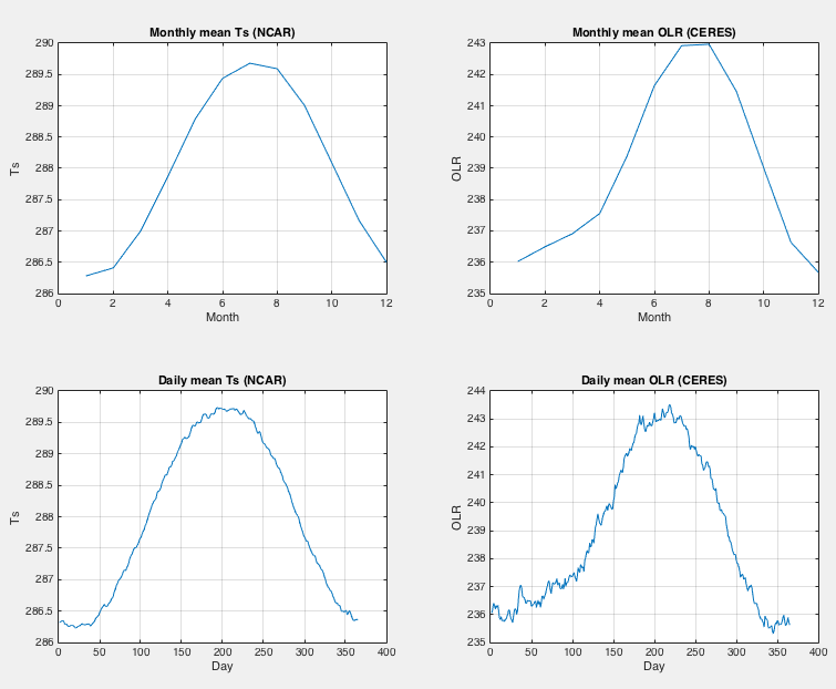
Figure 1
If we remove the monthly mean from the data, here are those same relationships (shown in the last article as anomalies from the overall 2001-2013 mean):

Figure 2 – Click to Expand
On a lag of 1 day there is a possible relationship with a low correlation – and the rest of the lags show no relationship at all.
Of course, we have created a problem with this new dataset – as the lag increases we are “jumping boundaries”. For example, on the 7-day lag all of the Ts data in the last week of April is being compared with the OLR data in the first week of May. With slowly rising temperatures, the last week of April will be “positive temperature data”, but the first week of May will be “negative OLR data”. So we expect 1/4 of our data to show the opposite relationship.
So we can show the data with the “monthly boundary jumps removed” – which means we can only show lags of say 1-14 days (with 3% – 50% of the data cut out); and we can also show the data as anomalies from the daily mean. Both have the potential to demonstrate the feedback on shorter timescales than the seasonal cycle.
First, here is the data with daily means removed:

Figure 3 – Click to Expand
Second, here is the data with the monthly means removed as in figure 2, but this time ensuring that no monthly boundaries are crossed (so some of the data is removed to ensure this):
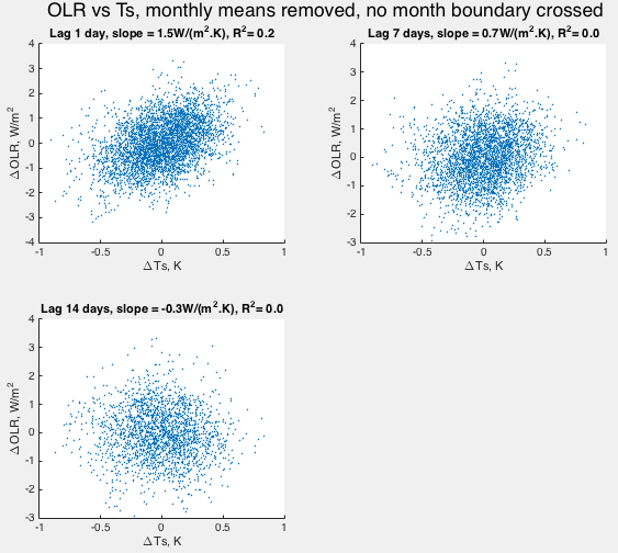
Figure 4 – Click to Expand
So basically this demonstrates no correlation between change in daily global OLR and change in daily global temperature on less than seasonal timescales. (Or “operator error” with the creation of my anomaly data). This is excluding (because we haven’t tested it here) the very short timescale of day to night change.
This was surprising at first sight.
That is, we see global Ts increasing on a given day but we can’t distinguish any corresponding change in global OLR from random changes, at least until we get to seasonal time periods? (See graph in last article).
Then what is probably the reason came into view. Remember that this is anomaly data (daily global temperature with monthly mean subtracted). This bar graph demonstrates that when we are looking at anomaly data, most of the changes in global Ts are reversed the next day, or usually within a few days:
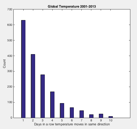
Figure 5
This means that we are unlikely to see changes in Ts causing noticeable changes in OLR unless the climate response we are looking for (humidity and cloud changes) occurs within a day or two.
That’s my preliminary thinking, looking at the data – i.e., we can’t expect to see much of a relationship, and we don’t see any relationship.
One further point – explained in much more detail in the (short) series Measuring Climate Sensitivity – is that of course changes in temperature are not caused by some mechanism that is independent of radiative forcing.
That is, our measurement problem is compounded by changes in temperature being first caused by fluctuations in radiative forcing (the radiation balance) and ocean heat changes and then we are measuring the “resulting” change in the radiation balance resulting from this temperature change:
Radiation balance & ocean heat balance => Temperature change => Radiation balance & ocean heat balance
So we can’t easily distinguish the net radiation change caused by temperature changes from the radiative contribution to the original temperature changes.
I look forward to readers’ comments.
Articles in the Series
Part One – introducing some ideas from Ramanathan from ERBE 1985 – 1989 results
Part One – Responses – answering some questions about Part One
Part Two – some introductory ideas about water vapor including measurements
Part Three – effects of water vapor at different heights (non-linearity issues), problems of the 3d motion of air in the water vapor problem and some calculations over a few decades
Part Four – discussion and results of a paper by Dessler et al using the latest AIRS and CERES data to calculate current atmospheric and water vapor feedback vs height and surface temperature
Part Five – Back of the envelope calcs from Pierrehumbert – focusing on a 1995 paper by Pierrehumbert to show some basics about circulation within the tropics and how the drier subsiding regions of the circulation contribute to cooling the tropics
Part Six – Nonlinearity and Dry Atmospheres – demonstrating that different distributions of water vapor yet with the same mean can result in different radiation to space, and how this is important for drier regions like the sub-tropics
Part Seven – Upper Tropospheric Models & Measurement – recent measurements from AIRS showing upper tropospheric water vapor increases with surface temperature
Part Eight – Clear Sky Comparison of Models with ERBE and CERES – a paper from Chung et al (2010) showing clear sky OLR vs temperature vs models for a number of cases
Part Nine – Data I – Ts vs OLR – data from CERES on OLR compared with surface temperature from NCAR – and what we determine
Part Ten – Data II – Ts vs OLR – more on the data


“That is, our measurement problem is compounded by changes in temperature being first caused by fluctuations in radiative forcing (the radiation balance) and ocean heat changes and then we are measuring the “resulting” change in the radiation balance resulting from this temperature change:
Radiation balance & ocean heat balance => Temperature change => Radiation balance & ocean heat balance
So we can’t easily distinguish the net radiation change caused by temperature changes from the radiative contribution to the original temperature changes.
I look forward to readers’ comments.
This in a nutshell is the problem with trying to diagnose feedback response using globally average data. It’s really hard to distinguish cause from effect or forcing from feedback. Looking at the hemispheres separately makes distinguishing cause and effect much clearer and easier.
Moreover, the net TOA flux change is what matters for diagnosing feedback. That is absorbed/reflected SW from the Sun and any change in OLR. Very tricky to accurately diagnose feedback since there is likely enough random internal variation that can cause changed in absorbed/reflected SW due a fluctuation albedo (in particular from clouds).
Any positive OLR value per K should be thought of as a negative feedback.
Temps go up, water vapor goes up (positive feedback), cloud cover declines (positive feedback), OLR goes up (negative feedback).
2 W/m2/K (negative OLR feedback) is equivalent to the water vapor positive feedback.
So that leaves clouds and a small albedo impact providing the positive feedbacks.
Missing Energy anyone? 3.33 W/m2 is missing right now.
0.66 W/m2/year energy accumulation rate versus 2.23 W/m2/year direct Forcing and 1.76 W/m2/year (feedbacks which are supposed to be showing up for a 0.75K temperature increase).
Bill Illis,
There is no missing energy, at least if you use sensitivity obtain from observational data. You left out the Planck feed back (Stephan-Boltzmann) which is something like -2.8 W/m^2 for the current warming of 0.85 K.
Well, I think you should add up the net forcing and the positive feedbacks expected and then tell me again that there is no missing energy.
0.66 W/m2/year versus 4.0 W/m2/year.
That equals “missing”.
If the Planck feedback is something that is expected, then why doesn’t the global warming prophesy include the Planck feedback as an “actual” feedback (which is actually no different that the OLR feedback we are talking about here).
The actual Planck feedback appears to be -3.34 W/m2/K (or there is an error in the forcing estimates and/or the positive feedback estimates, take your pick).
Bill Illis,
“I think you should add up the net forcing and the positive feedbacks expected and then tell me again that there is no missing energy”
One can not draw a correct conclusion from an incorrect calculation.
“If the Planck feedback is something that is expected, then why doesn’t the global warming prophesy include the Planck feedback as an “actual” feedback (which is actually no different that the OLR feedback we are talking about here).”
If you look in IPCC AR5 you will see that is exactly what they do. The Planck feedback is treated just like all the other feedbacks and the total feedback includes the Planck feedback.
If you look at the equation for simple energy balance models, you will see that the mathematically correct way to do the balance you suggest is to treat the Planck feedback like all the others.
There is a second way to define the terms (unhelpful in my opinion) in which there is a direct Stephan-Boltzmann response (Planck feedback) that produces a T change that is “amplified” by “feedbacks”. That is the definition you are using, but that definition is not consistent with your calculation.
Bill wrote: “Missing Energy anyone? 3.33 W/m2 is missing right now. 0.66 W/m2/year energy accumulation rate versus 2.23 W/m2/year direct Forcing and 1.76 W/m2/year (feedbacks which are supposed to be showing up for a 0.75K temperature increase).”
Is any heat really missing? Oversimplifying, an El Nino can be thought of as a transient reduction in upwelling of cold water from the deeper ocean in the eastern equatorial Pacific. The 97/98 El Nino increased GMST by 0.5 degC and the following La Nina reduced it by almost the same amount. When large short-term fluctuations in heat exchange between the surface and deeper ocean are possible, “missing heat” could easily be in the ocean below the mixed layer. Over a 15-year hiatus, an additional flux of 0.1 W/m2 below the mixed layer would create the appearance of 0.3 degC of “missing heat”. If the missing heat were concentrated just below the mixed layer (say 100-300 m), it would be detected by ARGO, but hasn’t been. Significant heat supposedly has been accumulating below 700 m during the hiatus, but this doesn’t make much sense to me and the observed change in temperature is tiny.
You may be mixing up a number of concepts: power, energy and temperature (how these are interconverted) and elsewhere radiative forcing and radiative imbalance.
SoD,
The assumption of linearity in OLR response to temperature should work pretty well over a few degrees change in temperature. However, recall that the composite plots that you are generating here include an “averaging in” of latitudes which undergo a seasonal change in daily average temperature of upto 40 K. Over these temperature ranges, it seems heroic to assume linear behaviour. Even the change in Planck response is non-linear over these ranges.
There are therefore at least two sources of noise:- (i) the OLR response to a plus X degrees change in the NH is not compensated for by a minus X degrees in the SH, because of the non-linearity of response (ii) the OLR response in the NH will generally have different atmospheric properties from its SH twin. So a perfect between-hemisphere compensation in temperature can still lead to a non-zero change in OLR, aka as confounding noise.
I suspect that to extract anything meaningful from these data would require, at the least, the assignment of properties to a latitude model.
SoD,
Further to the above, I have just carried out a very simple numerical experiment using a 5-zone model. Each of the zones has a sinusoidal temperature variation crudely approximating real Earth phasing and amplitude; the SH zones had a slightly smaller amplitude than the NH. Each zone was initialised at realistic temperatures, so that the. average Earth surface temperature worked out to be 288K by design. Total net peak-to-trough annual temperature variation worked out to be 3.4K, or +-1.7K around the average of 288k..
I then calculated for each zone, at time intervals throughout the year, the OLR predicted by S-B for that absolute temperature, and averaged the results over the zones (areally-weighted) to obtain an aggregate response. This gave me a cross-plot of aggregate OLR against average surface temperature. It is worthy of note that:-
(A) The cross-plot is multivalued because the same average temperature can be achieved by at least two combinations of temperature distributions.
(B) The OLS slope of the OLR vs temperature plot worked out to be only 86% of the theoretical value obtained by differentiating S-B and evaluating at the average temperature of 288k.
This approach assumes no feedbacks at all (save Planck), and no variation in response in different regions. I hope, however that its very simplicity serves to illustrate that the averaging problem is non-trivial.
I’ll second that. Clouds would add additional complication. I’m not at all sure that one could be confident from this data that a positive feedback exists.
Paul_K
You make an interesting point (sorry for my slow response).
Basically the “no feedback” result in your sample is not 3.6 W/m2 with the caveat that I’m not sure what result you calculated as the theoretical result – was it also 3.6 W/m2?
In Part Eight – Clear Sky Comparison of Models with ERBE and CERES we saw the calculation by Chung, Yeomans & Soden for a uniform 1K change in each location (top graph):
– and the global integration for this case results in 3.6 W/m2.
That is, the “no feedback” value was not calculated by a differentiation of the Stefan-Boltzmann equation in one case and hoping it stays the same (i.e., “linearity rules”), but instead by perturbing the average annual climatology by 1K everywhere and looking at the change in OLR. (Caveat – this case, the subject of their paper, is for clear sky conditions).
This first case I wanted to look at – the global case – is the only one that really makes sense to me.
Now someone else might calculate the global case by perturbing the annual mean climatology (or some other starting case) by different values and get a different “no feedback” case – that would be interesting to know and I might even be able to produce a set of values myself.
The problem with dividing results into latitude zones is the export of heat (and water vapor) across any arbitrary lines. About 1015W is exported from the equator to the poles, divided roughly half between the ocean and the atmosphere.
So if we calculate a value for 30S-30N, as an example, and we get ΔT(tropics) results in ΔOLR(tropics) what can we conclude?
In advance (I haven’t done the calculation yet) I’m not sure what value would indicate “no feedback”. We can pick the “boundary” of the Hadley circulation as our first boundary, but that is a moving feast. I downloaded GBs of data and figured out how to extract the data but I’m still unconvinced that I know how to interpret regional results.
SoD,
To me your response tells about the fact that no-feedback is not a concept that is naturally well defined. It’s actually a concept that can be defined well only referring to a model. Each model has its own definition of no-feedback as each model determines in a different way, what is considered a direct effect and what feedback. In a model no-feedback refers to the outcome when certain specific mechanisms are left out, but the rest of physics is as in the full model.
The real Earth has only changes that include feedbacks. If the reaction of the Earth to a sudden change could be determined as a function of time, changes over some short intervals might be close to no-feedback in some interpretation, but significant ambiguity would occur even in that.
The concept of no-feedback sensitivity can be used because typical full Earth system models do not differ quantitatively very much in their estimates of the no-feedback sensitivity.
Pekka,
It seems like a core component of physics is breaking apart problems into “unphysical” aka “model” problems to see what we can determine:
– “What happens when the beam rests on a perfect frictionless surface..”
– “The pendulum is a point mass on a rod of zero mass”
and so on.
“No feedback” does need more specification – to me it means that there is no change in the radiation balance due to changes in water vapor & clouds concentration/distribution, or due to ocean/atmospheric circulation changes. There will be subtly different descriptions of “no feedback” and the calculated value might depend upon the amount of the perturbation, the annual climatology and so on.
The version that I have seen used is the result of a uniform 1K increase in surface and atmosphere, where the surface & atmosphere temperatures are the annual mean values.
We could suggest it is the annual average of (1K increase in daily mean conditions). That is we produce the Jan 1 average, perturb by 1K, calculate the change. Produce the Jan 2 average, perturb by 1K, calculate the change. Etc. And average the results.
Or take the conditions each 6 hours over 1 year and average.
If the results are so variable based upon the perturbation, the averaging, or the climatology chosen then we might conclude it isn’t a useful value. I suspect the “no feedback” value doesn’t vary very much with the perturbation or the climatology, but I could be wrong.
I don’t expect that the climate has a real feedback (i.e. the result of all of the changes, including water vapor, clouds, circulation changes) that is a constant. That would be amazing if it were the case.
SoD,
A uniform 1K change is spectacularly unlikely to happen. Its only selling point is that it makes the calculation easier. In something more like the real world, the temperature increase should be higher at higher latitudes (polar amplification). That would also tend to flatten the latitudinal distribution of OLR.
I did realize the 1K everywhere is not a likely scenario.
So, if we wanted to test out the idea it would be a case of dusting off the radiative transfer model, put in some “standard atmospheres” for different regions and plot the W/m2 per K for different surface temperatures and temperature deviations (for constant absolute humidity).
So it would be a 3d plot showing ΔOLR/ΔT on surface temperature vs temperature deviation?
Something like that. You could have different levels of polar amplification that still gave a global average change of 1K, like the poles rising twice as fast as the tropics and four times as fast and compare with a uniform increase.. Then there would be the question of the interpolation function. You could have the the temperature be linear with latitude or perhaps with the sine of the latitude. My suspicion is that the ΔOLR would be greater with more polar amplification.
SoD,
Thanks for the response and the useful reminder of Chung et al.
You are raising a number of interesting questions. To avoid confusing the issues, let me here just address your first question, which was about what my calculation reveals, if anything.
My crude calculation suppresses diurnal variation, but allows “realistic” seasonal surface temperature variation (and phasing of such variation) in each of 5 latitude zones. I can express this variation either as absolute temperature variation or as variation in temperature anomaly. Using S-B (assumed emissivity of 1.0) together with the absolute values of surface temperature, I can calculate time series for surface-emitted OLR for each zone, and combine them in a weighted average to obtain a time series for variation in aggregate global OLR emitted from the surface.
This is of course not the same as the OLR emitted at TOA. In fact, the mean surface-emitted OLR works out to be about 396W/m^2 for this model. (This is slightly higher than the 390W/m^2 we would calculate by plugging the mean absolute temperature of the model into S-B.)
A cross-plot of the aggregate surface-emitted OLR against average temperature anomaly now produces an OLS gradient which is 4.7 W/m^2/degK. A black-body non-rotating billiard ball at a uniform temperature of 288K (the average temperature of the model) should produce a theoretical gradient of 5.4W/m^2/degK at that temperature. This latter gradient is very similar to a secant gradient estimated for a small uniform change of temperature across the whole planet. The first gradient is only 86% of the latter.
I do not claim that the 86% is correct in any sense. If I were to repeat the exercise and separate the land and ocean response in each of the latitude zones, I would obtain a different (and probably even lower) value for this ratio. My only point is that these gradient values are significantly different from each other. They are different because temperature anomaly is being averaged linearly, but the OLR response is a linear (weighted areal) average of a function which is responding in a non-linear way.
To be clear then, I am not claiming that this exercise reveals anything at all about feedbacks, or about OLR at TOA. I am claiming that it offers some limited insight into the spatio-temporal averaging process. This (among some other things which I wish to return to in a later comment) makes interpretation of your posted results problematic.
Your posted results include OLR at TOA. These values have already undergone a spatio-temporal averaging process which tested a (massive) change in both surface temperatures and brightness temperatures over the annual cycle. You cannot presume that your OLR vs dT gradient values have the same meaning that you might attribute to them if you were testing a billiard-ball model with a small uniform change in temperature.
I will offer a further post on the other interesting points you raise here.
SoD,
The ‘no-feedback’ TOA flux change for +1K for the clear sky should be a linear increase in aggregate dynamics to offset the post albedo input power for the clear sky.
Mainstream climate science considers a watt of incremental GHG absorption equal to a watt of incremental post albedo solar power entering in its intrinsic ability to further warm the surface (hence why each is said to have the same ‘no-feedback’ surface temperature increase). Even though I think this is highly dubious, shouldn’t the same convention be applied to a hypothetical clear sky only atmosphere?
How specifically again are they arriving at 3.6 W/m^2?
The more I think about it, the more I don’t think this exercise of looking at the clear sky by itself is valid at all, and that the ‘no-feedback’ TOA flux change only really makes sense when it includes clouds. Most of us know that it’s 3.3 W/m^2 per 1C of warming on global average, which includes the combined effects of the clear and cloudy skies.
Paul_K,
[fixed up after the fact, left and right brackets don’t work when typed in, as WordPress thinks they are html tags – anyone wanting to do it has to type “& lang ;” and “& rang ;” without the spaces]
I agree on the specific problem that I think you are raising (and I have written about this problem in various articles):
– if you average a set of data and apply a non-linear formula to that average value you get a different result than if you input all of the data into the formula and average the result.
That is:
x is a dataset: x1, x2, x3..xn
Z1 = f(⟨x⟩), where ⟨x⟩ is the mean of x1, x2, x3, etc
y = f(x), Z2 = ⟨y⟩, where ⟨y⟩ is the mean of y1, y2, y3, etc
Generally Z1 ≠ Z2
That isn’t how the 3.6 W/m2 was calculated – i.e., it wasn’t calculated from applying a formula to a global average.
It was calculated from an annual climatology (datapoints of latitude vs height) with a 1K perturbation at each point (surface and atmosphere) and seeing the OLR change.
The question that I think arises with the question of averaging in this specific case: does ΔOLR/ΔT (i.e. the change in W/m2 per 1K of temperature change) vary with the temperature perturbation we apply.
To put it in concrete terms:
– if we use 2K uniformly do we get the same graph?
– if we use 30K over continental land and 5K over the oceans do we get the same graph?
SoD,
Thank you for your post of July 17 9:43pm. It is always good when someone plays back what they have understood from a comment. You have grasped the main first point I was trying to make about the spatio-temporal averaging problem as it applies to interpretation of seasonal variation.
In addition to this averaging problem there are other significant confounding factors.
The seasonal variation in radiative flux and temperature are not solely controlled by the wave of insolation that passes over the planet during its annual orbit. There are at least three other known “Mexican waves” to be considered:-
a. An orbitally-driven annual and semi-annual momentum flux which causes oscillation in atmospheric circulation; this adds and subtracts energy as well as redistributing sensible heat in the mid- and upper- troposphere.
b. An albedo wave driven by recurrent seasonal changes in cloud, snow and ice distribution.
c. The cycle of shortwave absorption into the atmosphere relative to surface absorption. SW absorption is in phase with solar insolation, and on average over the annual cycle the atmosphere is more transparent than absorbing. Consequently, on average, the atmosphere is more heated by surface fluxes from below than by atmospheric absorption from above. From year to year, there is little net change in system energy, barring external forcing of the system. So it may be a reasonable assumption that the radiative fluxes are in long-term balance at TOA, and that total energy fluxes (including convection) are in balance at the surface ON AVERAGE. However, during the annual cycle, this assumption is completely invalid. Both locally and globally, there is a net gain and a net loss of system energy during the seasonal cycle. There is therefore no physical requirement that the SW absorption at the surface is balanced by upward energy fluxes from the surface; this is especially true over the oceans because of their heat capacity. The OLR at any given locale is therefore not driven just by the surface temperature at that locale, but is also driven by the variation in atmospheric heating over the seasonal cycle – which modifies the vertical temperature profile.
Each of these three waves changes the local relationship between surface temperature and OLR emission at TOA. The above seasonal changes are not effects which can be plausibly neglected. Yet, none of these three effects are present when we consider the question of radiative flux changes or feedbacks associated with interannual or decadal warming. The key question then becomes:- To what extent does the relationship between OLR and surface temperature evident during the annual cycle represent the relationship we might expect to see during a multiannual warming trend? The problem is that we do not know the answer to this question, but the true answer may be “very little or not at all”.
First, this data and post are awesome. It is something I’ve often wondered about. Thank you for the work.
While I couldn’t predict it, I am not surprised at the result because the air is thick with absorption in long IR wavelengths. You have shown that the material that makes up our atmosphere is basically black at these wavelengths which we sort of know but it is hard to understand. No I’m not the guy who thinks that proves the air is IR saturated or whatever nonsense. Is it possible to check the same at higher atmospheric altitudes? I actually don’t know which dataset that would be but it would almost certainly give an increased correlation and it might be fun.
very cool
SOD wrote: “So basically this demonstrates no correlation between change in daily global OLR and change in daily global temperature on less than seasonal timescales.”
Wouldn’t it be better to say that: So basically this demonstrates no correlation between change in daily global OLR ANOMALY and change in daily global temperature ANOMALY on less than seasonal timescales. The temperature anomaly varies within about +/-0.5 degK (0.2%) and the OLR anomaly varies within +/-2 W/m2 (0.8%). See the reference below for an alternative way to plot the monthly data. Note how tight the error bars are.
Click to access 7568.full.pdf
If the error in our ability to measure Ts and OLR is about this size, then the scatter plot simply represents noise.
Since most OLR originates well above the surface, your plots are asking how long it takes a surface temperature anomaly to propagate several to the characteristic emission altitude. If upward propagation takes one day in some regions, several days in other regions and several weeks in others, you won’t see much correlation at any lag. (Lag 0 is missing.)
To me, the concept of so-called ‘no-feedback’ should be a linear increase in aggregate dynamics (or a linear increase in adaption).
““No feedback” does need more specification – to me it means that there is no change in the radiation balance due to changes in water vapor & clouds concentration/distribution, or due to ocean/atmospheric circulation changes.”
I agree with this, but don’t agree it is the same for a watt of additional GHG absorption as it is for a watt of additional post albedo solar power entering the system. Of course, because in each case whether it’s +1 W/m^2 of post albedo solar power or +1 W/m^2 of GHG absorption, there will be a -1 W/m^2 TOA deficit that has to be restored, you can arbitrarily warm surface and atmosphere by the same amount needed to offset +1 W/m^2 post albedo solar power to restore balance for + 1 W/m^2 GHG absorption, but that’s trivially true.
But maybe this isn’t the right thread to discuss this.
Is it at least understood that mainstream climate science considers the intrinsic surface warming ability of a watt of post albedo solar power and a watt of GHG absorption to be the same? Because each is considered to have the same ‘no-feedback’ surface temperature increase?
RW,
It’s generally understood that different forcings have different effects, but it’s common to assume that these differences can be neglected as small. These differences are discussed in this 2005 paper by Hansen and 43 other authors.
Yeah, but the point I’m trying to get at is how intrinsic forcing is quantified. I certainly agree that anything that causes a TOA radiative imbalance forces the system in someway, by some amount. The question is what is the proper way to quantify the intrinsic surface warming ability of a particular forcing.
[ moderator’s note – and see request below – rest of comment held in storage, ready to place in thread of your choice]
RW,
Which one of the 10 threads that you have (unintentionally) hijacked with 10 – 100 comments that sound exactly like these would you like to continue your personal struggle at?
I can’t tell if you are still totally confused or still trying to evangelize everyone to your point of view – whatever that point of view is – and having responded to 100s of your comments in the past I definitely don’t want you to explain (again).
Please pick one of those threads – resume your discussion there and post one comment here to say “please join me on [thread] for continued discussion of [summary in 20 words or less of your mission].
RW,
I don’t think that the factor of 1.6 is used in the derivation. To the extent the factor is true it’s an outcome, not input.
“I don’t think that the factor of 1.6 is used in the derivation. To the extent the factor is true it’s an outcome, not input.”
The 1.6 factor really just quantifies the lapse rate, i.e. the effective temperature decrease from the surface to the TOA, relative to emitted IR power, and which is offsetting post albedo solar power. Or that it takes about 385 W/m^2 of net surface gain to allow 239 W/m^2 to leave the system at the TOA, offsetting the 239 W/m^2 of post albedo solar power absorbed That you can increase that linearly to offset incremental GHG absorption is of course true, but my point (or case at least) is doing so doesn’t really quantify a linear increase in aggregate dynamics offsetting GHG absorption and thus is not really an accurate measure of the intrinsic surface warming ability of GHG absorption.
That aside even, the second last paragraph in my last post makes the notion that a watt of GHG absorption and watt of post albedo solar power have equal intrinsic surface warming abilities highly dubious. BTW, I’m assuming everyone agrees that if each is claimed to have the same ‘no-feedback’ surface temperature increase, than it’s effectively being claimed that the intrinsic surface warming ability of each is equal to one another.
SoD,
“I can’t tell if you are still totally confused or still trying to evangelize everyone to your point of view – whatever that point of view is – and having responded to 100s of your comments in the past I definitely don’t want you to explain (again).”
Well, it’s certainly possible I could still be confused, but I may not be either. I can’t remember what threads some of these things were (I guess) discussed on. Maybe a post of yours that deals entirely with the notion of so-called ‘no-feedback’ would be worthwhile. Or if there already is one, perhaps that would be the best place to have this discussion, as I agree it’s really largely off the topic of this thread.
OK, let’s continue this discussion here:
SOD and Paul_K: The subject of the last post – seasonal changes in outgoing OLR and SWR associated with the 3.5 degC increase in MGST – is great for demonstrating that climate models are both wrong and inconsistent representing feedbacks except for WV+LR (OLR from clear skies). Unfortunately seasonal warming (NH – SH) is a poor model for global warming because the NH and SH are so different, especially in ocean and cloud coverage. Seasonal changes can tell us about how well or poorly models perform, but not the magnitude of feedbacks during global warming. However, “global feedbacks” are the sum of regional feedbacks. As SOD notes, you can’t analyze regional feedbacks only with Ts and outgoing CERES data – you need to correct for meridional transport of heat and worrying about non-linearity. These appears to be a far more tractable problems than dealing with errors in measuring changes is GMST and radiative flux on a decadal time scale and dealing with unforced variability. Those problems appear hopeless. It’s far better to have a strong, but complicated, signal (3.5 degC warming globally, up to 40 degC locally) that repeats every year than a simpler weak signal observed with a differing array of instruments at most once a decade.
If I understand correctly, Figure 3 from Dessler, J Climate (2013) provides evidence that feedbacks vary dramatically with latitude (and IMO probably terrain: ocean, coastal, continental).
Click to access dessler2013.pdf
Shindell’s paper attempting to discredit energy balance models asserts that climate models show that aerosol forcing, which is regional, is more effective at changing Ts than the global forcing from GHGs.
Frank,
I have a comment in moderation which addresses in more detail the problem of comparing the seasonal cycle with multiannual warming. (It is in moderation, I think, because I didn’t understand SoD’s previous instruction concerning brackets. I do now. I hope that SoD will accept my apology for my repeat stupidity here, and let the comment out of moderation.)
I agree with much of what you say. In particular, I think it would be a truly valuable exercise to try to produce a model which did fully match the seasonal variation in terms of heat fluxes, radiative fluxes, atmospheric momentum and temperature. I suspect that this would reveal some shortfalls in the physics we are currently assuming in AOGCMs. However, I also think that this is a mammoth undertaking. At present, none of the GCMs have the capability to match heat and momentum fluxes at regional level. Nor can they reproduce well the amplitude of temperature variation by latitude. it would require the building of a new type of model or major modifications to an existing model.
I also believe however that if the objective is solely to gain insight into radiative feedbacks from the seasonal data, then there is a halfway house which needs radiative code, but which avoids the need for phenomenological modelling. This requires characterisation from the observational data (i.e. prescription), for a specified number of zones, of the data required to calculate and match the local OLR. Heat fluxes (including atmospheric meridonial heat fluxes) can be prescribed rather than calculated. This is less likely to reveal any serious problems with the physics, but once a match had been achieved, LW feedbacks regionally and in aggregate could be assessed by perturbation from the local mean behaviour. This is still a large task, but one which would be somewhat easier than, and a natural precursor to, building and matching a new phenomelogical model.
Paul, thanks for your patience with comments in moderation.
Actually it is not me putting them there, it is WordPress. I use hosted WordPress and wonderful though it is, it decides for reasons I don’t understand that a comment is suspect.
All explained in Comments & Moderation
Paul_K: Thanks for the reply. I hope an answer to some model problems is already available in the output from ensembles of models. If we looked, could we find several parameter sets that perform better at reproducing the seasonal cycle or some other set of observables (TCR from energy balance models)? I gather from the work of Stainforth et al that a large number of parameter sets perform about as well (or badly, if you prefer) at reproducing today’s climate. Tuning parameters one by one appears to have left us in a featureless wilderness of minor local optima with no hope of finding a global optimum – except systematic exploration of all parameter space motivated by confronting the worst failures of modeling. Limitations associated with the size of grid cells could frustrate such a search, but even that problem would be more tractable if simulations could be run for several years rather than several decades or centuries.
The recent discussion reminds me of the comment of Ramanathan quoted in the first post of this series:
Pekka,
Your comment prompted me to re-read some comments I made on the same subject 5 years ago. It was embarrassing for me in that, on that thread, I went all round the houses to prove something which I could have done far more simply and more generally. What I wanted to show was that, under the same billiard ball Earth assumption as made by Ramanathan, the derivative w.r.t surface temp of G as defined by Ramanathan relates to the TOTAL FEEDBACK of the system, and not just the LW feedbacks. I will include a simple proof below. Given this, I still find Ramanathan’s conclusion to be unsafe, when he asserts “The analysis confirms…” The furthest he should have gone was to state that the overall feedback (including the seasonal effects of heat transfer and SW absorption change) appeared to be positive relative to Planck – under some non-trivial assumptions.
Simple proof for billiard-ball Earth follows (this assumes no error introduced by spatio-temporal averaging).
Transient net flux behaviour at TOA can be textually stated as:- change in net flux from steady-state at t= 0 is equal to the change in input flux minus the change in outgoing flux:-
ΔN(t) = ΔI(t) – ΔO(t)
.The only outgoing flux is LW. Making the common approximation that this can be expressed as a linear function of surface temperature (as does Ramanathan), we have
ΔO(t) = OLR(t) – OLR(0) = λ*ΔTs = λ*(Ts(t) – Ts(0)) (1)
where λ is the TOTAL FEEDBACK term.
differentiating (1) w.r.t. Ts, we obtain:-
d(OLR)/dTs = λ (2)
Ramanathan defines G for all-sky from the relationship:-
OLR = σTs^4 – G (3)
Differentiating (3) we obtain:-
d(OLR)/dTs = 4σTs^3 – dG /dTs (4)
Substitute (2) and we obtain:-
dG/dTs = 4σTs^3 – λ (5)
Equations (2) and (5) both indicate that the response that Ramanathan is testing must include all feedbacks. This includes the effect on the vertical temperature profile of the variation in shortwave heating via atmospheric absorption. I think it is a stretch to believe that the water vapour feedback can be isolated from these data, even though Ramanathan’s conclusion of positive feedback may turn out to be correct.
[…] « Clouds & Water Vapor – Part Ten – Data II – Ts vs OLR […]