In Latent heat and Parameterization I showed a formula for calculating latent heat transfer from the surface into the atmosphere, as well as the “real” formula. The parameterized version has horizontal wind speed x humidity difference (between the surface and some reference height in the atmosphere, typically 10m) x “a coefficient”.
One commenter asked:
Why do we expect that vertical transport of water vapor to vary linearly with horizontal wind speed? Is this standard turbulent mixing?
The simple answer is “almost yes”. But as someone famously said, make it simple, but not too simple.
Charting a course between too simple and too hard is a challenge with this subject. By contrast, radiative physics is a cakewalk. I’ll begin with some preamble and eventually get to the destination.
There’s a set of equations describing motion of fluids and what they do is conserve momentum in 3 directions (x,y,z) – these are the Navier-Stokes equations, and they conserve mass. Then there are also equations to conserve humidity and heat. There is an exact solution to the equations but there is a bit of a problem in practice. The Navier-Stokes equations in a rotating frame can be seen in The Coriolis Effect and Geostrophic Motion under “Some Maths”.
Simple linear equations with simple boundary conditions can be re-arranged and you get a nice formula for the answer. Then you can plot this against that and everyone can see how the relationships change with different material properties or boundary conditions. In real life equations are not linear and the boundary conditions are not simple. So there is no “analytical solution”, where we want to know say the velocity of the fluid in the east-west direction as a function of time and get a nice equation for the answer. Instead we have to use numerical methods.
Let’s take a simple problem – if you want to know heat flow through an odd-shaped metal plate that is heated in one corner and cooled by steady air flow on the rest of its surface you can use these numerical methods and usually get a very accurate answer.
Turbulence is a lot more difficult due to the range of scales involved. Here’s a nice image of turbulence:
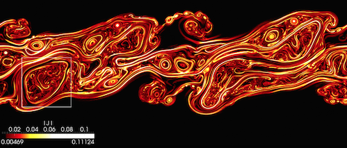
From NASA – http://www.nas.nasa.gov/SC12/demos/demo28.html
Figure 1
There is a cascade of energy from the largest scales down to the point where viscosity “eats up” the kinetic energy. In the atmosphere this is the sub 1mm scale. So if you want to accurately numerically model atmospheric motion across a 100km scale you need a grid size probably 100,000,000 x 100,000,000 x 10,000,000 and solving sub-second for a few days. Well, that’s a lot of calculation. I’m not sure where turbulence modeling via “direct numerical simulation” has got to but I’m pretty sure that is still too hard and in a decade it will still be a long way off. The computing power isn’t there.
Anyway, for atmospheric modeling you don’t really want to know the velocity in the x,y,z direction (usually annotated as u,v,w) at trillions of points every second. Who is going to dig through that data? What you want is a statistical description of the key features.
So if we take the Navier-Stokes equation and average, what do we get? We get a problem.
For the mathematically inclined the following is obvious, but of course many readers aren’t, so here’s a simple example:
Let’s take 3 numbers: 1, 10, 100: the average = (1+10+100)/3 = 37.
Now let’s look at the square of those numbers: 1, 100, 10000: the average of the square of those numbers = (1+100+10000)/3 = 3367.
But if we take the average of our original numbers and square it, we get 37² = 1369. It’s strange but the average squared is not the same as the average of the squared numbers. That’s non-linearity for you.
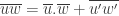
In the Navier Stokes equations we have values like east velocity x upwards velocity, written as uw. The average of uw, written as 

When we create the Reynolds averaged Navier-Stokes (RANS) equations we get lots of new terms like
It’s like saying x + y = 1, what is x and y? No one can say. Perhaps 1 & 0. Perhaps 1000 & -999.
Digression on RANS for Slightly Interested People
The Reynolds approach is to take a value like u,v,w (velocity in 3 directions) and decompose into a mean and a “rapidly varying” turbulent component.
So 


And
So in the original equation where we have a term like 
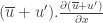

So 2 unknowns instead of 1. The first term is the averaged flow, the second term is the turbulent flow. (Well, it’s an advection term for the change in velocity following the flow)
When we look at the conservation of energy equation we end up with terms for the movement of heat upwards due to average flow (almost zero) and terms for the movement of heat upwards due to turbulent flow (often significant). That is, a term like 
Or, in plainer English, how heat gets moved up by turbulence.
..End of Digression
Closure and the Invention of New Ideas
“Closure” is a maths term. To “close the equations” when we have more unknowns that equations means we have to invent a new idea. Some geniuses like Reynolds, Prandtl and Kolmogoroff did come up with some smart new ideas.
Often the smart ideas are around “dimensionless terms” or “scaling terms”. The first time you encounter these ideas they seem odd or just plain crazy. But like everything, over time strange ideas start to seem normal.
The Reynolds number is probably the simplest to get used to. The Reynolds number seeks to relate fluid flows to other similar fluid flows. You can have fluid flow through a massive pipe that is identical in the way turbulence forms to that in a tiny pipe – so long as the viscosity and density change accordingly.
The Reynolds number, Re = density x length scale x mean velocity of the fluid / viscosity
And regardless of the actual physical size of the system and the actual velocity, turbulence forms for flow over a flat plate when the Reynolds number is about 500,000. By the way, for the atmosphere and ocean this is true most of the time.
Kolmogoroff came up with an idea in 1941 about the turbulent energy cascade using dimensional analysis and came to the conclusion that the energy of eddies increases with their size to the power 2/3 (in the “inertial subrange”). This is usually written vs frequency where it becomes a -5/3 power. Here’s a relatively recent experimental verification of this power law.
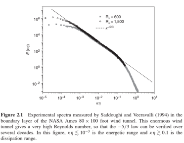
From Durbin & Reif 2010
Figure 2
In less genius like manner, people measure stuff and use these measured values to “close the equations” for “similar” circumstances. Unfortunately, the measurements are only valid in a small range around the experiments and with turbulence it is hard to predict where the cutoff is.
A nice simple example, to which I hope to return because it is critical in modeling climate, is vertical eddy diffusivity in the ocean. By way of introduction to this, let’s look at heat transfer by conduction.
If only all heat transfer was as simple as conduction. That’s why it’s always first on the list in heat transfer courses..
If have a plate of thickness d, and we hold one side at temperature T1 and the other side at temperature T2, the heat conduction per unit area:

where k is a material property called conductivity. We can measure this property and it’s always the same. It might vary with temperature but otherwise if you take a plate of the same material and have widely different temperature differences, widely different thicknesses – the heat conduction always follows the same equation.
Now using these ideas, we can take the actual equation for vertical heat flux via turbulence:

where w = vertical velocity, θ = potential temperature
And relate that to the heat conduction equation and come up with (aka ‘invent’):

Now we have an equation we can actually use because we can measure how potential temperature changes with depth. The equation has a new “constant”, K. But this one is not really a constant, it’s not really a material property – it’s a property of the turbulent fluid in question. Many people have measured the “implied eddy diffusivity” and come up with a range of values which tells us how heat gets transferred down into the depths of the ocean.
Well, maybe it does. Maybe it doesn’t tell us very much that is useful. Let’s come back to that topic and that “constant” another day.
The Main Dish – Vertical Heat Transfer via Horizontal Wind
Back to the original question. If you imagine a sheet of paper as big as your desk then that pretty much gives you an idea of the height of the troposphere (lower atmosphere where convection is prominent).
It’s as thin as a sheet of desk size paper in comparison to the dimensions of the earth. So any large scale motion is horizontal, not vertical. Mean vertical velocities – which doesn’t include turbulence via strong localized convection – are very low. Mean horizontal velocities can be the order of 5 -10 m/s near the surface of the earth. Mean vertical velocities are the order of cm/s.
Let’s look at flow over the surface under “neutral conditions”. This means that there is little buoyancy production due to strong surface heating. In this case the energy for turbulence close to the surface comes from the kinetic energy of the mean wind flow – which is horizontal.
There is a surface drag which gets transmitted up through the boundary layer until there is “free flow” at some height. By using dimensional analysis, we can figure out what this velocity profile looks like in the absence of strong convection. It’s logarithmic:
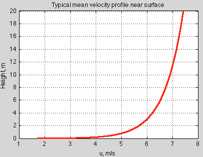
Figure 3 – for typical ocean surface
Lots of measurements confirm this logarithmic profile.
We can then calculate the surface drag – or how momentum is transferred from the atmosphere to the ocean – using the simple formula derived and we come up with a simple expression:

Where Ur is the velocity at some reference height (usually 10m), and CD is a constant calculated from the ratio of the reference height to the roughness height and the von Karman constant.
Using similar arguments we can come up with heat transfer from the surface. The principles are very similar. What we are actually modeling in the surface drag case is the turbulent vertical flux of horizontal momentum 
Adding the Richardson number for non-neutral conditions we end up with a temperature difference along with a reference velocity to model the turbulent vertical flux of sensible heat 

Now with a bit more maths..
At the surface the horizontal velocity must be zero. The vertical flux of horizontal momentum creates a drag on the boundary layer wind. The vertical gradient of the mean wind, U, can only depend on height z, density ρ and surface drag.
So the “characteristic wind speed” for dimensional analysis is called the friction velocity, u*, and

This strange number has the units of velocity: m/s – ask if you want this explained.
So dimensional analysis suggests that 
So a simple re-arrangement and integration gives:

where z0 is a constant from the integration, which is roughness height – a physical property of the surface where the mean wind reaches zero.
The “real form” of the friction velocity is:

we can pick a horizontal direction along the line of the mean wind (rotate coordinates) and come up with:

If we consider a simple constant gradient argument:

where the first expression is the “real” equation and the second is the “invented” equation, or “our attempt to close the equation” from dimensional analysis.
Of course, this is showing how momentum is transferred, but the approach is pretty similar, just slightly more involved, for sensible and latent heat.
Conclusion
Turbulence is a hard problem. The atmosphere and ocean are turbulent so calculating anything is difficult. Until a new paradigm in computing comes along, the real equations can’t be numerically solved from the small scales needed where viscous dissipation damps out the kinetic energy of the turbulence up to the large scale of the whole earth, or even of a synoptic scale event. However, numerical analysis has been used a lot to test out ideas that are hard to test in laboratory experiments. And can give a lot of insight into parts of the problems.
In the meantime, experiments, dimensional analysis and intuition have provided a lot of very useful tools for modeling real climate problems.