In Eleven – End of the Last Ice age we saw the sequence of events that led to the termination of the most recent ice age – Termination I.
The date of this event, the time when the termination began, was about 17.5-18.0 kyrs ago (note 1). We also saw that “rising solar insolation” couldn’t explain this. By way of illustration I produced some plots in Pop Quiz: End of An Ice Age – all from the last 100 yrs and asked readers to identify which one coincided with Termination I.
But this simple graph of insolation at 65ºN on July 1st summarizes the problem for the”classic version” (see Part Six – “Hypotheses Abound”) of the “Milankovitch theory” – in simple terms, if solar insolation at 18 kyrs ago caused the ice age to end, why didn’t the same or higher insolation at 100 kyrs, 80 kyrs, or from 60-30 kyrs cause the last ice age to end earlier:

Figure 1
And for a more visual demonstration of solar insolation changes in time, take a look at the Hövmoller plots in the comments of Part Eleven.
The other problem for the Milankovitch theory of ice age termination is the fact that southern hemisphere temperatures rose in advance of global temperatures. So the South led the globe out of the ice age. This is hard to explain if the cause of the last termination was melting northern hemisphere ice sheets. Take a look at Eleven – End of the Last Ice age.
Now we’ve quickly reviewed Termination I, let’s take a look at Termination II. This is the end of the penultimate ice age.
The traditional Milankovitch theory says that peak high latitude solar insolation around 127 kyrs BP was the trigger for the massive deglaciation that ended that earlier ice age.
The well-known SPECMAP dating of sea-level/ice-volume vs time has Termination II at 128 ± 3 kyrs BP. All is good.
Or is it?
What is the basis for the SPECMAP dating?
The ice age records that have been most used and best known come from ocean sediments. These were the first long-dated climate records that went back hundreds of thousands of years.
How do they work and what do they measure?
Oxygen exists in the form of a few different stable isotopes. The most common is 16O with 18O the next most common, but much smaller in proportion. Water, aka H2O, also exists with both these isotopes and has the handy behavior of evaporating and precipitating H218O water at different rates to H216O. The measurement is expressed as the ratio (the delta, or δ) as δ18O in parts per thousand.
The journey of water vapor evaporating from the ocean, followed by precipitation, produces a measure of the starting ratio of the isotopes as well as the local precipitation temperature.
The complex end result of these different process rates is that deep sea benthic foraminifera take up 18O out of the deep ocean, and the δ18O ratio is mostly in proportion to the global ice volume. The resulting deep sea sediments are therefore a time-series record of ice volume. However, sedimentation rates are not an exact science and are not necessarily constant in time.
As a result of lots of careful work by innumerable people over many decades, out popped a paper by Hays, Imbrie & Shackleton in 1976. This demonstrated that a lot of the recorded changes in ice volume happened at orbital frequencies of precession and obliquity (approximately every 20kyrs and every 40 kyrs). But there was an even stronger signal – the start and end of ice ages – at approximately every 100 kyrs. This coincides roughly with changes in eccentricity of the earth’s orbit, not that anyone has a (viable) theory that links this change to the start and end of ice ages.
Now the clear signal of obliquity and precession in the record gives us the option of “tuning up” the record so that peaks in the record match orbital frequencies of precession and obliquity. We discussed the method of tuning in some past comments on a similar, but much later, dataset – the LR04 stack (thanks to Clive Best for highlighting it).
The method isn’t wrong, but we can’t confirm the timing of key events with a dataset where dates have been tuned to a specific theory.
Luckily, some new methods have come along.
Ice Core Dating
It’s been exciting times for the last twenty plus years in climate science for people who want to wear thick warm clothing and “get away from it all”.
Greenland and Antarctica have yielded a number of ice cores. Greenland now has a record that goes back 123,000 years (NGRIP). Antarctica now has a record that goes back 800,000 years (EDC, aka, “Dome C”). Antarctica also has the Voskok ice core that goes back about 400,000 years, Dome Fuji that goes back 340,000 years and Dronning Maud Land (aka DML or EDML) which is higher resolution but only goes back 150,000 years.
What do these ice cores measure and how is the dating done?
The ice cores measure temperature at time of snow deposition via the δ18O measurement discussed above (note 2), which in this case is not a measure of global ice volume but of air temperature. The gas trapped in bubbles in the ice cores gives us CO2 and CH4 concentrations. We also can measure dust deposition and all kinds of other goodies.
The first problem is that the gas is “younger” than the ice because it moves around until the snow compacts enough. So we need a model to calculate this, and there is some uncertainty about the difference in age between the ice and the gas.
The second problem is how to work out the ice age. At the start we can count annual layers. After sufficient time (a few tens of thousands of years) these layers can’t be distinguished any more, instead we can use models of ice flow physics. Then a few handy constraints arrive like 10Be events that occurred about 50 kyrs BP. After ice flow physics and external events are exhausted, the data is constrained by “orbital tuning”, as with deep ocean cores.
Caves, Corals and Accurate Radiometric Dating
Neither deep sea cores, nor ice cores, give us much possibility of radiometric dating. But caves and corals do.
For newcomers to dating methods, if you have substance A that decays into substance B with a “half-life” that is accurately known, and you know exactly how much of substance A and B was there at the start (e.g. no possibility of additional amounts of A or B getting into the thing we want to measure) then you can very accurately calculate the age that the substance was formed.
Basically it’s all down to how to deposition process works. Uranium-Thorium dating has been successfully used to date calcite depositions in rock.
So, take a long section that has been continuously deposited, measure the δ18O (and 13C) at lots of points along the section, and take a number of samples and calculate the age along the section with radiometric dating. The subject of what exactly is being measured in the cores is complicated, but I will greatly over-simplify and say it revolves around two points:
- The actual amount of deposition, as not much water is available to create these depositions during extreme glaciation
- The variation of δ18O (and 13C), which to a first order depends on local air temperature
For people interested in more detail, I recommend McDermott 2004, some relevant extracts below in note 3).
Corals offer the possibility, via radiometric dating, of getting accurate dates of sea level. The most important variable to know is any depression and uplift of the earth’s crust.
Accurate dating of caves and coral has been a growth industry in the last twenty years with some interesting results.
Termination II
Winograd et al 1992 analyzed Devils Hole in Nevada (DH-11):
The Devils Hole δ18O time curve (fig 2) clearly displays the sawtooth pattern characteristic of marine δ18O records that have been interpreted to be the result of the waxing and waning of Northern Hemisphere ice sheets.. But what caused the δ18O variations in DH-11 shown on fig. 2? ..The δ18O variations in atmospheric precipitation are – to a first approximation – believed to reflect changes in average winter-spring surface temperature..

From Winograd et al 1992
Figure 2
Termination II occurs at 140±3 (2σ) ka in the DH-11 record, at 140± 15 ka in the Vostok record (14), and at 128 ± 3 ka in the SPECMAP record (13). (The uncertainty in the DH-11 record is in the 2σ uncertainties on the MS uranium-series dates; other dates and uncertainties are from the sources cited.) Termination III occurred at about 253 +/- 3 (2σ) ka in the DH11 record and at about 244 +/- 3 ka in the SPECMAP record. These differences.. are minimum values..
They compare summer insolation at 65ºN with SPECMAP, Devils Hole and the Vostok ice core on a handy graph:

Winograd et al 1992
Figure 3
Of course, not everyone was happy with this new information, and who knows what the isotope measurement really was a proxy for?
Slowey, Henderson & Curry 1996
A few years later, in 1996, Slowey, Henderson & Curry (not the famous Judith) made this statement from their research:
Our dates imply a timing and duration for substage 5e in substantial agreement with the orbitally tunes marine chronology. Initial direct U-Th dating of the marine δ18O record supports the theory that orbital variations are a fundamental cause of Pleistocene climate change.
[Emphasis added, likewise with all quotes].
Henderson & Slowey 2000
Then in 2000, the same Henderson & Slowey (sans Curry):
Milankovitch proposed that summer insolation at mid-latitudes in the Northern Hemisphere directly causes the ice-age climate cycles. This would imply that times of ice-sheet collapse should correspond to peaks in Northern Hemisphere June insolation.
But the penultimate deglaciation has proved controversial because June insolation peaks 127 kyr ago whereas several records of past climate suggest that change may have occurred up to 15kyr earlier.
There is a clear signature of the penultimate deglaciation in marine oxygen-isotope records. But dating this event, which is significantly before the 14C age range, has not been possible.
Here we date the penultimate deglaciation in a record from the Bahamas using a new U-Th isochron technique. After the necessary corrections for a-recoil mobility of 234U and 230Th and a small age correction for sediment mixing, the midpoint age for the penultimate deglaciation is determined to be 135 +/-2.5 kyr ago. This age is consistent with some coral-based sea-level estimates, but it is difficult to reconcile with June Northern Hemisphere insolation as the trigger for the ice-age cycles.
Zhao, Xia & Collerson (2001)
High-precision 230Th- 238U ages for a stalagmite from Newdegate Cave in southern Tasmania, Australia.. The fastest stalagmite growth occurred between 129.2 ± 1.6 and 122.1 ± 2.0 ka (61.5 mm/ka), coinciding with a time of prolific coral growth from Western Australia (128-122 ka). This is the first high-resolution continental record in the Southern Hemisphere that can be compared and correlated with the marine record. Such correlation shows that in southern Australia the onset of full interglacial sea level and the initiation of highest precipitation on land were synchronous. The stalagmite growth rate between 129.2 and 142.2 ka (5.9 mm/ka) was lower than that between 142.2 and 154.5 ka (18.7 mm/ka), implying drier conditions during the Penultimate Deglaciation, despite rising temperature and sea level.
This asymmetrical precipitation pattern is caused by latitudinal movement of subtropical highs and an associated Westerly circulation, in response to a changing Equator-to-Pole temperature gradient.
Both marine and continental records in Australia strongly suggest that the insolation maximum between 126 and 128 ka at 65°N was directly responsible for the maintenance of full Last Interglacial conditions, although the triggers that initiated Penultimate Deglaciation (at 142 ka) remain unsolved.
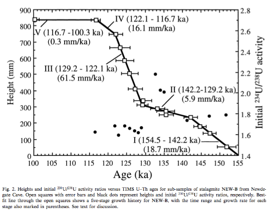
From Zhao et al 2001
Figure 4
Gallup, Cheng, Taylor & Edwards (2002)
An outcrop within the last interglacial terrace on Barbados contains corals that grew during the penultimate deglaciation, or Termination II. We used combined 230Th and 231Pa dating to determine that they grew 135.8 ± 0.8 thousand years ago, indicating that sea level was 18 ± 3 meters below present sea level at the time. This suggests that sea level had risen to within 20% of its peak last- interglacial value by 136 thousand years ago, in conflict with Milankovitch theory predictions..
Figure 2B summarizes the sea level record suggested by the new data. Most significantly our record includes corals that document sea level directly during Termination II, suggesting that the majority (~80%) of the Termination II sea level rise occurred before 135 ka. This is broadly consistent with early shifts in δ18O recorded in the Bahamas and Devils Hole and with early dates (134 ka) of last interglacial corals from Hawaii, which call into question the timing of Termination II in the SPECMAP record..
From Gallup et al 2002
Figure 5 – Click to expand
Of course, all is not lost for the many-headed Hydra (and see note 4):
..The Milankovitch theory in its simplest form cannot explain Termination II, as it does Termination I. However, it is still plausible that insolation forcing played a role in the timing of Termination II. As deglaciations must begin while Earth is in a glacial state, it is useful to look at factors that could trigger deglaciation during a glacial maximum. These include – (i) sea ice cutting off a moisture source for the ice sheets; – (ii) isostatic depression of continental crust; and – (iii) high Southern Hemisphere summer insolation through effects on the atmospheric CO concentration.
Yuan et al 2004 provide evidence in opposition:
Thorium-230 ages and oxygen isotope ratios of stalagmites from Dongge Cave, China, characterize the Asian Monsoon and low-latitude precipitation over the past 160,000 years. Numerous abrupt changes in 18O/16O values result from changes in tropical and subtropical precipitation driven by insolation and millennial-scale circulation shifts.
The Last Interglacial Monsoon lasted 9.7 +/- 1.1 thousand years, beginning with an abrupt (less than 200 years) drop in 18O/16O values 129.3 ± 0.9 thousand years ago and ending with an abrupt (less than 300 years) rise in 18O/16O values 119.6 ± 0.6 thousand years ago. The start coincides with insolation rise and measures of full interglacial conditions, indicating that insolation triggered the final rise to full interglacial conditions.
But they also comment:
Although the timing of Monsoon Termination II is consistent with Northern Hemisphere insolation forcing, not all evidence of climate change at about this time is consistent with such a mechanism (Fig. 3).
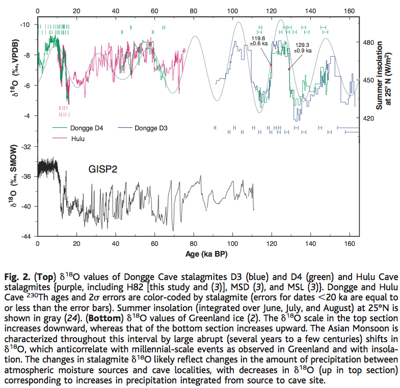
From Yuan et al 2004
Figure 6 – Click to expand
Sea level apparently rose to levels as high as –21 m as early as 135 ky before the present (27 & Gallup et al 2002), preceding most of the insolation rise. The half-height of marine oxygen isotope Termination II has been dated at 135 +/- 2.5 ky (Henderson & Slowey 2000).
Speleothem evidence from the Alps indicates temperatures near present values at 135 +/- 1.2 ky (31). The half-height of the d18O rise at Devils Hole (142 +/- 3 ky) also precedes most of the insolation rise (20). Increases in Antarctic temperature and atmospheric CO2 (32) at about the time of Termination II appear to have started at times ranging from a few to several millennia before most of the insolation rise (4, 32, 33).
[Their reference numbers amended to papers where cited in this article]
Drysdale et al 2009
Variations in the intensity of high-latitude Northern Hemisphere summer insolation, driven largely by precession of the equinoxes, are widely thought to control the timing of Late Pleistocene glacial terminations. However, recently it has been suggested that changes in Earth’s obliquity may be a more important mechanism. We present a new speleothem-based North Atlantic marine chronology that shows that the penultimate glacial termination (Termination II) commenced 141,000 ± 2,500 years before the present, too early to be explained by Northern Hemisphere summer insolation but consistent with changes in Earth’s obliquity. Our record reveals that Terminations I and II are separated by three obliquity cycles and that they started at near-identical obliquity phases.
Standard stuff by now, for readers who have made it this far.
But the Drysdale paper is interesting on two fronts – their dating method and their “one result in a row” matching a theory with evidence (I extracted more text from the paper in note 5 for interested readers). Let’s look at the dating method first.
Basically what they did was match up the deep ocean cores that record global ice volume (but have no independent dating) with accurately radiometrically-dated speleothems (cave depositions). How did they do the match up? It’s complicated but relies on the match between the δ18O in both records. The approach of providing absolute dating for existing deep ocean cores will give very interesting results if it proves itself.

From Drysdale et al 2009
Figure 7 – Click to expand
The correspondence between Corchia δ18O and Iberian-margin sea-surface temperatures (SSTs) through T-II (Fig. 2) is remarkable. Although the mechanisms that force speleothem δ18O variations are complex, we believe that Corchia δ18O is driven largely by variations in rainfall amount in response to changes in regional SSTs. Previous studies from Corchia show that speleothem δ18O is sensitive to past changes in North Atlantic circulation at both orbital and millennial time scales, with δ18O increasing during colder (glacial or stadial) phases and the reverse occurring during warmer (inter- glacial or interstadial) phases.

From Drysdale et al 2009
Figure 8 – Click to expand
Now to the hypothesis:

From Drysdale et al 2009
Figure 9
We find that NHSI [NH summer insolation] intensity is unlikely to be the driving force for T-II: Intensity values are close to minimum at the time of the start of T-II, and a lagged response to the previous insolation peak at ~148 ka is unlikely because of its low amplitude (Fig. 3A). This argues against the SPECMAP curve being a reliable age template through T-II, given the age offset of ~8 ky for the T-II midpoint (8) with respect to our record. A much stronger case can be made for obliquity as a forcing mechanism.
On the basis of our results (Fig. 3B), both T-I and T-II commence at the same phase of obliquity, and the period between them is exactly equivalent to three obliquity cycles (~123 ky).
(More of their explanation in note 5).
EPICA 2006
Here is my plot of the Dronning Maud Land ice core (DML) on EDC3 timescale from EPICA 2006 (data downloaded from the Nature website):
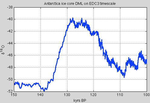
Data from EPICA
Figure 10
The many Antarctic and Greenland ice cores are still undergoing revisions of dating, and so I haven’t attempted to get the latest work. I just thought it would be good to throw in an ice core.
The value of δ18O here is a proxy for local temperature. On this timescale local temperatures began rising about 138 kyrs BP.
Conclusion
New data on Termination II from the last 20 years of radiometric dating from a number of different sites with different approaches demonstrate that TII started about 140 kyrs BP.
Here is the solar insolation curve at 65ºN over the last 180 kyrs, with the best dates of the two ice age terminations, separated by about 121 – 125 kyrs:

Figure – Click to expand
It’s proven that ice ages are terminated by low solar insolation in the high latitudes of the northern hemisphere. The basis for this is that the low solar insolation allows a much quicker build up of the northern hemisphere ice sheets, causing dynamic instability, leading to ice sheet calving, which disrupts ocean currents, outgassing CO2 in large concentrations and thereby creating a positive feedback for temperature rise. The local ice sheet collapses also create positive feedback due to higher solar insolation now absorbed. As the ice sheets continue to melt, the (finally) rising solar insolation in high northern latitudes strengthens the pre-existing conditions and helps to establish the termination. Thus the orbital theory is given strong support from the evidence of the timing of the last two terminations.
I just made that up in a few minutes for fun. It’s not true.
We saw one paper with different evidence for the start of TII – Yuan et al (and see note 6). However, it seems that most lines of evidence, including absolute dating of sea level rise puts TII starting around 140 kyrs BP.
This also means, for maths wizards, that the time between ice age terminations, from one result in a row, is about 122 kyrs.
As an aside, because Winograd et al 1992 calculated their age for TIII “at about 253 kyrs”:
This puts the time between TIII and TII at about 113 kyrs which is exactly the time of five precessional cycles!
I haven’t yet dug into any other dates for TIII so this theory is quite preliminary.
Articles in the Series
Part One – An introduction
Part Two – Lorenz – one point of view from the exceptional E.N. Lorenz
Part Three – Hays, Imbrie & Shackleton – how everyone got onto the Milankovitch theory
Part Four – Understanding Orbits, Seasons and Stuff – how the wobbles and movements of the earth’s orbit affect incoming solar radiation
Part Five – Obliquity & Precession Changes – and in a bit more detail
Part Six – “Hypotheses Abound” – lots of different theories that confusingly go by the same name
Part Seven – GCM I – early work with climate models to try and get “perennial snow cover” at high latitudes to start an ice age around 116,000 years ago
Part Seven and a Half – Mindmap – my mind map at that time, with many of the papers I have been reviewing and categorizing plus key extracts from those papers
Part Eight – GCM II – more recent work from the “noughties” – GCM results plus EMIC (earth models of intermediate complexity) again trying to produce perennial snow cover
Part Nine – GCM III – very recent work from 2012, a full GCM, with reduced spatial resolution and speeding up external forcings by a factors of 10, modeling the last 120 kyrs
Part Ten – GCM IV – very recent work from 2012, a high resolution GCM called CCSM4, producing glacial inception at 115 kyrs
Pop Quiz: End of An Ice Age – a chance for people to test their ideas about whether solar insolation is the factor that ended the last ice age
Eleven – End of the Last Ice age – latest data showing relationship between Southern Hemisphere temperatures, global temperatures and CO2
Twelve – GCM V – Ice Age Termination – very recent work from He et al 2013, using a high resolution GCM (CCSM3) to analyze the end of the last ice age and the complex link between Antarctic and Greenland
Fourteen – Concepts & HD Data – getting a conceptual feel for the impacts of obliquity and precession, and some ice age datasets in high resolution
Fifteen – Roe vs Huybers – reviewing In Defence of Milankovitch, by Gerard Roe
Sixteen – Roe vs Huybers II – remapping a deep ocean core dataset and updating the previous article
Seventeen – Proxies under Water I – explaining the isotopic proxies and what they actually measure
Eighteen – “Probably Nonlinearity” of Unknown Origin – what is believed and what is put forward as evidence for the theory that ice age terminations were caused by orbital changes
Nineteen – Ice Sheet Models I – looking at the state of ice sheet models
References
A Pliocene-Pleistocene stack of 57 globally distributed benthic D18O records, Lorraine E. Lisiecki & Maureen E. Raymo, Paleoceanography (2005) – free paper
Continuous 500,000-Year Climate Record from Vein Calcite in Devils Hole, Nevada, Winograd, Coplen, Landwehr, Riggs, Ludwig, Szabo, Kolesar & Revesz, Science (1992) – paywall, but might be available with a free Science registration
Palaeo-climate reconstruction from stable isotope variations in speleothems: a review, Frank McDermott, Quaternary Science Reviews 23 (2004) – free paper
Direct U-Th dating of marine sediments from the two most recent interglacial periods, NC Slowey, GM Henderson & WB Curry, Nature (1996)
Evidence from U-Th dating against northern hemisphere forcing of the penultimate deglaciation, GM Henderson & NC Slowey, Nature (2000)
Timing and duration of the last interglacial inferred from high resolution U-series chronology of stalagmite growth in Southern Hemisphere, J Zhao, Q Xia & K Collerson, Earth and Planetary Science Letters (2001)
Direct determination of the timing of sea level change during Termination II, CD Gallup, H Cheng, FW Taylor & RL Edwards, Science (2002)
Timing, Duration, and Transitions of the Last Interglacial Asian Monsoon, Yuan, Cheng, Edwards, Dykoski, Kelly, Zhang, Qing, Lin, Wang, Wu, Dorale, An & Cai, Science (2004)
Evidence for Obliquity Forcing of Glacial Termination II, Drysdale, Hellstrom, Zanchetta, Fallick, Sánchez Goñi, Couchoud, McDonald, Maas, Lohmann & Isola, Science (2009)
One-to-one coupling of glacial climate variability in Greenland and Antarctica, EPICA Community Members, Nature (2006)
Millennial- and orbital-scale changes in the East Asian monsoon over the past 224,000 years, Wang, Cheng, Edwards, Kong, Shao, Chen, Wu, Jiang, Wang & An, Nature (2008)
Notes
Note 1 – In common ice age convention, the date of a termination is the midpoint of the sea level rise from the last glacial maximum to the peak interglacial condition. This can be confusing for newcomers.
Note 2 – The alternative method used on some of the ice cores is δD, which works on the same basis – water with the hydrogen isotope Deuterium evaporates and condenses at different rates to “regular” water.
Note 3 – A few interesting highlights from McDermott 2004:
2. Oxygen isotopes in precipitation
As discussed above, d18O in cave drip-waters reflect
(i) the d18O of precipitation (d18Op) and
(ii) in arid/semi- arid regions, evaporative processes that modify d18Op at the surface prior to infiltration and in the upper part of the vadose zone.
The present-day pattern of spatial and seasonal variations in d18Op is well documented (Rozanski et al., 1982, 1993; Gat, 1996) and is a consequence of several so-called ‘‘effects’’ (e.g. latitude, altitude, distance from the sea, amount of precipitation, surface air temperature).
On centennial to millennial timescales, factors other than mean annual air temperature may cause temporal variations in d18Op (e.g. McDermott et al., 1999 for a discussion). These include:
(i) changes in the d18O of the ocean surface due to changes in continental ice volume that accompany glaciations and deglaciations;
(ii) changes in the temperature difference between the ocean surface temperature in the vapour source area and the air temperature at the site of interest;
(iii) long-term shifts in moisture sources or storm tracks;
(iv) changes in the proportion of precipitation which has been derived from non-oceanic sources, i.e. recycled from continental surface waters (Koster et al., 1993); and
(v) the so-called ‘‘amount’’ effect.
As a result of these ambiguities there has been a shift from the expectation that speleothem d18Oct might provide quantitative temperature estimates to the more attainable goal of providing precise chronological control on the timing of major first-order shifts in d18Op, that can be interpreted in terms of changes in atmospheric circulation patterns (e.g. Burns et al., 2001; McDermott et al., 2001; Wang et al., 2001), changes in the d18O of oceanic vapour sources (e.g. Bar Matthews et al., 1999) or first-order climate changes such as D/O events during the last glacial (e.g. Spo.tl and Mangini, 2002; Genty et al., 2003)..
4.1. Isotope stage 6 and the penultimate deglaciation
Speleothem records from Late Pleistocene mid- to high-latitude sites are discussed first, because these are likely to be sensitive to glacial–interglacial transitions, and they illustrate an important feature of speleothems, namely that calcite deposition slows down or ceases during glacials. Fig. 1 is a compilation of approximately 750 TIMS U-series speleothem dates that have been published during the past decade, plotted against the latitude of the relevant cave site.
The absence of speleothem deposition in the mid- to high latitudes of the Northern Hemisphere during isotope stage 2 is striking, consistent with results from previous compilations based on less precise alpha-spectrometric dates (e.g. Gordon et al., 1989; Baker et al., 1993; Hercmann, 2000). By contrast, speleothem deposition appears to have been essentially continuous through the glacial periods at lower latitudes in the Northern Hemisphere (Fig. 1)..
..A comparison of the DH-11 [Devils Hole] record with the Vostok (Antarctica) ice-core deuterium record and the SPEC- MAP record that largely reflects Northern Hemisphere ice volume (Fig. 2) indicates that both clearly record the first-order glacial–interglacial transitions.
Note 4 – Note the reference to Milankovitch theory “explaining” Termination I. This appears to be the point that insolation was at least rising as Termination began, rather than falling. It’s not demonstrated or proven in any way in the paper that Termination I was caused by high latitude northern insolation, it is an illustration of the way the “widely-accepted point of view” usually gets a thumbs up. You can see the same point in the quotation from the Zhao paper. It’s the case with almost every paper.
If it’s impossible to disprove a theory with any counter evidence then it fails the test of being a theory.
Note 5 – More from Drysdale et al 2009:
During the Late Pleistocene, the period of glacial-to-interglacial transitions (or terminations) has increased relative to the Early Pleistocene [~100 thousand years (ky) versus 40 ky]. A coherent explanation for this shift still eludes paleoclimatologists. Although many different models have been proposed, the most widely accepted one invokes changes in the intensity of high-latitude Northern Hemisphere summer insolation (NHSI). These changes are driven largely by the precession of the equinoxes, which produces relatively large seasonal and hemispheric insolation intensity anomalies as the month of perihelion shifts through its ~23-ky cycle.
Recently, a convincing case has been made for obliquity control of Late Pleistocene terminations, which is a feasible hypothesis because of the relatively large and persistent increases in total summer energy reaching the high latitudes of both hemispheres during times of maximum Earth tilt. Indeed, the obliquity period has been found to be an important spectral component in methane (CH4) and paleotemperature records from Antarctic ice cores.
Testing the obliquity and other orbital-forcing models requires precise chronologies through terminations, which are best recorded by oxygen isotope ratios of benthic foraminifera (d18Ob) in deep-sea sediments (1, 8).
Although affected by deep-water temperature (Tdw) and composition (d18Odw) variations triggered by changes in circulation patterns (9), d18Ob signatures remain the most robust measure of global ice-volume changes through terminations. Unfortunately, dating of marine sediment records beyond the limits of radiocarbon methods has long proved difficult, and only Termination I [T-I, ~18 to 9 thousand years ago (ka)] has a reliable independent chronology.
Most marine chronologies for earlier terminations rely on the SPECMAP orbital template (8) with its a priori assumptions of insolation forcing and built-in phase lags between orbital trigger and ice-sheet response. Although SPECMAP and other orbital-based age models serve many important purposes in paleoceanography, their ability to test climate- forcing hypotheses is limited because they are not independent of the hypotheses being tested. Consequently, the inability to accurately date the benthic record of earlier terminations constitutes perhaps the single greatest obstacle to unraveling the problem of Late Pleistocene glaciations..
..
Obliquity is clearly very important during the Early Pleistocene, and recently a compelling argument was advanced that Late Pleistocene terminations are also forced by obliquity but that they bridge multiple obliquity cycles. Under this model, predominantly obliquity-driven total summer energy is considered more important in forcing terminations than the classical precession-based peak summer insolation model, primarily because the length of summer decreases as the Earth moves closer to the Sun. Hence, increased insolation intensity resulting from precession is offset by the shorter summer duration, with virtually no net effect on total summer energy in the high latitudes. By contrast, larger angles of Earth tilt lead to more positive degree days in both hemispheres at high latitudes, which can have a more profound effect on the total summer energy received and can act essentially independently from a given precession phase. The effect of obliquity on total summer energy is more persistent at large tilt angles, lasting up to 10 ky, because of the relatively long period of obliquity. Lastly, in a given year the influence of maximum obliquity persists for the whole summer, whereas at maximum precession early summer positive insolation anomalies are cancelled out by late summer negative anomalies, limiting the effect of precession over the whole summer.
Although the precise three-cycle offset between T-I and T-II in our radiometric chronology and the phase relationships shown in Fig. 3 together argue strongly for obliquity forcing, the question remains whether obliquity changes alone are responsible.
Recent work invoked an “insolation-canon,” whereby terminations are Southern Hemisphere–led but only triggered at times when insolation in both hemispheres is increasing simultaneously, with SHSI approaching maximum and NHSI just beyond a minimum. However, it is not clear that relatively low values of NHSI (at times of high SHSI) should play a role in deglaciation. An alternative is an insolation canon involving SHSI and obliquity.
Note 6 – There are a number of papers based on Dongge and Hulu caves in China that have similar data and conclusions but I am still trying to understand them. They attempt to tease out the relationship between δ18O and the monsoonal conditions and it’s involved. These papers include: Kelly et al 2006, High resolution characterization of the Asian Monsoon between 146,000 and 99,000 years B.P. from Dongge Cave, China and global correlation of events surrounding Termination II; Wang et al 2008, Millennial- and orbital-scale changes in the East Asian monsoon over the past 224,000 years.


Winograd et al 1992 comment in their paper:
SoD,
I have been following this excellent series with great interest, but can’t claim to be keeping up with all the nuances. Can I offer a summary of what I think I’ve understood to date for your comment?
I’ll start by quoting AR4 FAQ 6.1 as the “standard” model:
As I read your series, the following strikes me:
1)It does seem pretty much certain that orbital changes are linked to the ice age cycle in some way
2)However, it is not possible to be certain exactly how – there are many differing theories.
3)The uncertainty is greater with deglaciations compared to onset of glaciation
4)The uncertainty is compounded by the difficulty in aging proxy records, and these are tuned to the known orbital cycle in many presentations (this came as a surprise me).
5)It is even plausible that deglaciations in particular are not actually correlated to orbital changes at all, but are a result of the inherent dynamics of the system.
6)GCMs are some way from being able to quantitatively predict the onset of glaciations or deglaciations.
My take-home is that the certainty implied in the standard model is overstated.
Is this broadly your take? Anything here you’d disagree with?
many thanks for this great resource.
verytallguy,
It is a challenging subject (for everyone), and keeping up with the nuances is difficult.
Let me respond to your points in line.
Yes, but the nuance here is important.
The waxing and waning of ice sheets is clearly linked to the obliquity and precession of the earth’s orbit around the sun. But the start and end of ice ages (ice age “inception” and ice age “termination”) are not clearly linked to the orbital changes.
If you like this is the biggest part of the problem in the “standard theory” – these two are interlinked in the description, but not in any physics.
Picture, if you will, two completely separate and unrelated theories:
– Theory A – ice sheets expand and contract with a strong connection to obliquity and precession
– Theory B – ice ages start and end due to something related to orbital changes
Theory A has strong support.
Theory B has little support (and evidence against).
But because in common climate science thinking there is a theory that combines Theory A & B, when doubt is cast on Theory B, the proponents push out some evidence for Theory A in support of Theory B.
Hopefully the answer to 1 answers this question.
This is a working hypothesis for me at the moment, inspired by the comment of DeWitt Payne who pointed out that the earth seems to easily slip into glacials, and therefore the question is why the ice ages end, not why they start. However, I haven’t tried to line up a decent amount of evidence for this so I can’t claim any basis for the hypothesis.
I can see that the physics expressed via current climate models provides a some support for ice age inception due to low solar insolation in high latitudes, but it’s early days. Watch this space.
The tuning of the proxy records obscures the subject quite a bit, how much I can’t say.
Part of the reason why I can’t say is that proxy records in deep ocean cores capture a record of “global ice volume” in an undated time-series while better dated records capture a different proxy signal. So the solution is still not clear.
Hopefully, this article has “detuned” the proxy records in our minds as far as ice age terminations are concerned.
Possible, I haven’t really written about this yet, but it is plausible – to me. Plausible is a subjective term.
Basic work on chaotic systems teaches us that non-linear systems with a forcing term can show frequency responses of much longer timescales, and slip between different modes for “no reason” (“no reason” in a deterministic sense).
Let’s say that terminations/deglaciations do not have a known cause. Even if, for sake of argument, we said it was “inherent dynamics” or “stochastic resonance” or “chaos” we still have no explanation for a number of tightly linked processes – of which, the CO2 vs Antarctic/global temperatures are one of the biggest mysteries.
There are other mysteries as well. So it seems premature to claim “unstable dynamics” as the solution when we don’t understand some of the basic physics/chemistry/biology.
Correct, GCMs cannot predict deglaciations unless they have the key feedbacks (ice sheets, GHGs) prescribed as an input. Even then there are limited studies on deglaciations so I find it hard to comment today.
GCMs might be able to “predict” glaciations, but it is early days.
My reservation on “predict glaciations” is that when you know the answer, finding the result is a lot easier than when you don’t know the answer.
So if we set the bar at the lowest point – bring me your GCMs and show me a glacial inception – we might claim success.
If we set the bar at the next threshold – bring me your GCMs, show me your glacial inception and show me the GCM not predicting colder than normal everywhere in the high latitudes, and show me what your GCM produces at 140 kyrs BP when there was supposed to be a termination – we might find failure.
verytallguy,
In reference to the statements in the IPCC reports on paleoclimate, I recently had a couple of quick rereads of AR4 and AR5 draft (“Do Not Cite, Quote or Distribute”) but can’t yet comment on whether they represent this complex subject correctly, incorrectly but in line with a mass of overconfident peer-reviewed papers, or just over-confidently.
The IPCC reports will be the subject of one article in the future. Watch this space.
Thank you, in particular I hadn’t unuderstood your clarification under the first point. I’ll continue to follow the series with interest, but my lack of expertise precludes my adding much of value in the comments.
Obviously whilst paleoclimate is inherently interesting to the curious, there is also a pressing need to understand the future trajectory of climate from current conditions and with anthropogenic forcing.
The key quantification of that is climate sensitivity – an unsatisfactory linear metric given the nonlinearilty and instability shown here, but nevertheless probably as good a metric as it’s possible to think of.
It strikes me that qualitatively, the instability shown in all this paleoclimate glaciation data is a strong argument against low sensitivity. I suppose that is not necessarily translated to future climate where we are considering sensitivity in a regime with lower ice sheet area than during past glaciations, and therefore differnt albedo and circulation.
My understanding is that climate sensitivity estimates based on paleoclimate are using the “stable” climate conditions during a glacial maximum to constrain models rather than considering the dynamics of shifts. I may well be wrong though.
I wonder
(i) if you’d agree with the contention that the instability shown suggests relatively high climate sensitivity
(ii) if it is possible to quantify this in any meaningful way.
verytallguy,
I don’t know the answer to this. Certainly the huge climatic changes in the past indicate that at certain points there are strong positive feedbacks. This equals high climate sensitivity.
But we haven’t descended into snowball earth or fiery Venus. Why not? This indicates strong negative feedbacks somewhere. Low climate sensitivity?
The problem with identifying climate sensitivity is the idea that there is a such a value that can be produced.
Here is a useful quote from Cloud Feedbacks in the Climate System: A Critical Review, Stephens, Journal of Climate (2005):
Suppose, as a wild idea, that the climate has a different response to a given forcing, or perturbation, depending on the current climate state.
It’s not that we can’t work out the answer “value of climate sensitivity, S = X”, where X is a constant, it is that we are not asking the right question.
My own thoughts on climate sensitivity is we can only measure a value, or provide a climate sensitivity, S = f(a,b,c,d,e..) if we happen to understand climate.
Otherwise we are just picking two points on a time series chart and calculating the change between those two points and dividing by another change. If you take the climate as shown in many different graphs in this series and pick 10 pairs of points at random over different timescales you will get 10 completely different answers to climate sensitivity.
To be discussed later in the series I hope.
The free link for the Stephens paper cited above – well worth reading.
SoD,
thanks again, interesting. I’ve had a quick look at the Stephens paper you recommend, and rapidly concluded that I’m out of my depth without spending a lot more time on this. No surprise there. I might try again later.
The strong negative feedback mitigating against snowball/Venus is, I presume, Stefan-Boltzmann.
Your
was what I’d expected.
Looking forward to the rest of the series
VTG
[…] uClimate.com is proving a real boom. I came across this article at Scienceofdoom. I can’t remember which way they swing on the debate, but the article is well written and a subject I’m interested in. Available at: https://scienceofdoom.com/2014/01/23/ghosts-of-climates-past-thirteen-terminator-ii/ […]
SOD: Have you read about other possible explanations for the termination (and/or initiation) of ice ages besides insolation at 65 degN? Do you intend to discuss any here?
Frank,
The two clusters of ideas on terminations that I have found so far:
1. Something to do with orbital variations
2. We have no idea what terminates ice ages
There are probably more ideas out there, but nothing has “stuck” as a viable hypothesis.
The reason that (1) has stuck as an idea is possibly because of (2).
Any idea – i.e., idea (1) – is better than no idea – i.e., idea (2) – to most people.
I provided some more termination dates from another paper in the discussion on another article and as it’s very relevant, I reproduce it here:
Winograd et al 1992 is cautious on dates for Termination IV and V due to radiometric uncertainties, but given that other dates (methods of dating) are uncertain, here is a figure from Duration and Structure of the Past Four Interglaciations, Winograd et al (1997):
This paper is specifically about the duration of interglacials, interesting in its own right, but identifies the termination date graphically.
(From Note 1 above, In common ice age convention, the date of a termination is the midpoint of the sea level rise from the last glacial maximum to the peak interglacial condition. This can be confusing for newcomers.)
I identify from the graph:
T-II – 142
T-III – 253
T-IV – 339
T-V – 418
T-VI – 520 (no identifying line for this termination)
This gives us (with TI as 18 kyrs, but perhaps it should be slightly later in time as we are considering the midpoints)
I-II = 124
II-III = 111
III-IV = 86
IV-V = 79
V-VI = 102
The average, no surprise, is 100 kyrs.
Here’s figure 5 from the same paper:
Click for a larger view
Now I’m going to take the time of termination as the time when the proxy measurement really started to increase:
T-II – 154
T-III – 269
T-IV – 354
T-V – 434
T-VI – 522 (taken from figure 2)
The period between the start of terminations:
[corrected, thanks to Arthur Smith]
I-II = 136 (taking the start of TI as about 18kyrs)
II-III = 115
III-IV = 85
IV-V = 80
V-VI = 88
[this following comment is now wrong] The average is 91 kyrs. The last period is clearly the aberration, and the average of the earlier 4 periods is 85 kyrs, which is exactly 4 precessional cycles! Problem solved.
With a small number of irregular periods you can pretty much make up whatever astrology you want..
It will be interesting to see how Dome C (EDC) from Antarctica compares. However, I believe there is some SPECMAP type tuning applied to older records (deeper parts of the core). I am still trying to understand the data.
Hi SoD – your subtraction of I-II, II-III and III-IV for start of terminations here seems wrong – from the numbers you gave for initiation it should be
I-II – 134 (?)
II-III – 115
III-IV – 85
Arthur,
Thanks, you are correct – my values are all out of line, with the first one missing. I will update the comment.
Now updating the average of the last 5 periods when we use the start of terminations – it is 101 kyrs.
In the paper:
A depth-derived Pleistocene age model: Uncertainty estimates, sedimentation variability, and nonlinear climate change, Peter Huybers & Carl Wunsch, Paleoceanography (2004), Huybers and Wunsch come up with an ocean δ18O vs age timeseries.
This is developed without assuming anything about the orbital theory:
Emphasis added. The B-M transition is the Matuyama–Brunhes geomagnetic reversal.
The assumptions include a model of depth compaction, and an assumption that the transitions between different cores all represent the same time:
Click to expand
I don’t have the dataset but have emailed Peter Huybers to ask for it.
SoD,
Have you checked the data link on Peter Huybers home page?
My first impression is that the data is available there.
Peter Huybers replied to my email:
Maybe the closing of Panama set off a persistent oscillation.
If I remember correctly, planetary hothouse conditions are all marked by not having land masses at the equator so the principal ocean circulation is equatorial, not polar. The current pattern of ocean gyres would seem to be warming high latitudes at the expense of the tropics. But in fact, they act to cool the entire planet over time and the high latitudes cool faster than the tropics.
Right. Tethys closing during the Oligocene was also a big feature that may have triggered permanent Antarctic glaciation.
DeWitt wrote: “The current pattern of ocean gyres would seem to be warming high latitudes at the expense of the tropics. But in fact, they act to cool the entire planet over time and the high latitudes cool faster than the tropics.”
I was intrigued by these statements and wanted to be sure I understood them. From a purely mathematical perspective, the T^4 factor in S-B plays a role. If the surface were uniformly 288 degK, it would radiate 390.1 W/m2. If it were half 273 degK and half 303 degK (averaging 288 degK), it would radiate 396.4 W/m2 – so we need some cooling. Half 271.83 degK and half 301.83 degK (averaging 286.83 degK or 1.17 degK less) would do the job. However, I suspect this may not be what you had in mind.
If the tropics did not export as much heat to cooler regions via ocean currents, how would it get rid of the extra heat? Radiative cooling is very inefficient due to the high humidity, so increased convection appears to be the logical route. That gets the excess heat high enough that it can escape via radiative cooling. Is this what you had in mind?
Frank,
It’s a lot more complicated than that. What counts is the local balance of radiation at the TOA, compared to absorption of incoming solar radiation and the resulting energy transport to achieve global radiative balance. There will always be an excess of absorption of incoming radiation compared to outgoing radiation at low latitudes and the opposite at high latitudes, so there will always be latitudinal energy transport. But if you have a steady state and then increase latitudinal energy transport, you’ve created an energy leak which over hundreds of thousands of years will cool the whole planet, and conversely.
That probably didn’t help much. Obviously I don’t have all the details worked out. And it’s somewhat counter-intuitive that there would be less energy transfer when the average surface temperature was higher.
DeWitt:”And it’s somewhat counter-intuitive that there would be less energy transfer when the average surface temperature was higher.”
Now I’m confused. I thought your point was that tectonic configurations controlled ocean energy transfers and climate regimes. You now seem to be saying that climate regimes control energy transfers.
I thought that your point was the lateral energy isolation restricted to the tropics due to an absence of continental blockages and a strong Coriolis force was responsible for hotter climate. Alternatively, once the tropical ocean current gates closed when the continental land masses become connected throughout the tropics and temperate zones, the forced longitudinal ocean currents leads to tropical heat transport toward the poles with subsequent discharge to space.
I always thought this was the commonly understood explanation of mid to late Cenozoic cooling shift
Howard,
I don’t think I said that at all.
[…] 2014/01/23: TSoD: Ghosts of Climates Past – Thirteen – Terminator II […]
DeWitt wrote above: “But if you have a steady state and then increase latitudinal energy transport, you’ve created an energy leak which over hundreds of thousands of years will cool the whole planet, and conversely.”
Isn’t the only “energy leak” that is important to the whole planet, the pathway to space, not internal energy transport? That’s why my comment focused cooling via larger fluxes to space.
Frank,
I thought I made it clear, but obviously I didn’t. The energy leak is to space and would be caused by an increase in area corrected TOA emission at high latitude greater than the decrease in area corrected TOA emission at low latitudes while absorption of incoming radiation remained the same. This change would be the direct result of a change in energy transport from low to high latitude at the surface.
Thanks, DeWitt it’s all clear to me now and makes perfect sense. My poor reading comprehension strikes again.
Frank, maybe if you think of the gulf stream, that would be helpful. The wiki page has some nice graphics. If the isthmus of Panama was open (as it was >~4-Myr ago) , much of this tropical Atlantic heat would be transported into the tropical Pacific instead of deflecting north to Greenland where some of it is radiated to space.
Here is where DeWitt’s point finally sinks in with me: It’s counter-intuitive that glacial advances would be initiated by transporting more heat to the north pole.
Howard,
I doubt that your reading comprehension is entirely or even mostly to blame. What seems clear to me isn’t always clear to others.
That’s what I thought I said, but your phrasing makes it much clearer. Pekka is really good at stating things clearly and elegantly too.
DeWitt and Howard: Thanks. In my first comment, I imagined a world where transport of heat was so efficient that the planet had a uniform temperature of 288 degK. Then I compared it to a planet with less effective transport of heat producing a “tropical zone” about 30 degK warmer than a polar zone. More polar transport of heat must cause some cooling, but the change seems small to me.
Frank,
Try including obliquity in your model. With no seasons I wouldn’t expect the temperature distribution to make much difference either. Also, what are your assumptions for the atmosphere? If you’re just looking at a spherical surface with no atmosphere, there won’t be much effect either. The lower temperature and resulting lower specific humidity at the poles means that the addition of one joule of energy at the pole will cause a larger temperature increase than at the equator, assuming constant relative humidity.
DeWitt: I agree with: “one joule of energy at the pole will cause a larger temperature increase than at the equator”. Is it wrong to call this “Arctic amplification”?
[…] Thirteen – Terminator II – looking at the date of Termination II, the end of the penultimate ice age – and implications for the cause of Termination II […]
[…] https://scienceofdoom.com/2014/01/23/ghosts-of-climates-past-thirteen-terminator-ii/ […]