In Ensemble Forecasting we had a look at the principles behind “ensembles of initial conditions” and “ensembles of parameters” in forecasting weather. Climate models are a little different from weather forecasting models but use the same physics and the same framework.
A lot of people, including me, have questions about “tuning” climate models. While looking for what the latest IPCC report (AR5) had to say about ensembles of climate models I found a reference to Tuning the climate of a global model by Mauritsen et al (2012). Unless you work in the field of climate modeling you don’t know the magic behind the scenes. This free paper (note 1) gives some important insights and is very readable:
The need to tune models became apparent in the early days of coupled climate modeling, when the top of the atmosphere (TOA) radiative imbalance was so large that models would quickly drift away from the observed state. Initially, a practice to input or extract heat and freshwater from the model, by applying flux-corrections, was invented to address this problem. As models gradually improved to a point when flux-corrections were no longer necessary, this practice is now less accepted in the climate modeling community.
Instead, the radiation balance is controlled primarily by tuning cloud-related parameters at most climate modeling centers while others adjust the ocean surface albedo or scale the natural aerosol climatology to achieve radiation balance. Tuning cloud parameters partly masks the deficiencies in the simulated climate, as there is considerable uncertainty in the representation of cloud processes. But just like adding flux-corrections, adjusting cloud parameters involves a process of error compensation, as it is well appreciated that climate models poorly represent clouds and convective processes. Tuning aims at balancing the Earth’s energy budget by adjusting a deficient representation of clouds, without necessarily aiming at improving the latter.
A basic requirement of a climate model is reproducing the temperature change from pre-industrial times (mid 1800s) until today. So the focus is on temperature change, or in common terminology, anomalies.
It was interesting to see that if we plot the “actual modeled temperatures” from 1850 to present the picture doesn’t look so good (the grey curves are models from the coupled model inter-comparison projects: CMIP3 and CMIP5):

From Mauritsen et al 2012
Figure 1
The authors state:
There is considerable coherence between the model realizations and the observations; models are generally able to reproduce the observed 20th century warming of about 0.7 K..
Yet, the span between the coldest and the warmest model is almost 3 K, distributed equally far above and below the best observational estimates, while the majority of models are cold-biased. Although the inter-model span is only one percent relative to absolute zero, that argument fails to be reassuring. Relative to the 20th century warming the span is a factor four larger, while it is about the same as our best estimate of the climate response to a doubling of CO2, and about half the difference between the last glacial maximum and present.
They point out that adjusting parameters might just be offsetting one error against another..
In addition to targeting a TOA radiation balance and a global mean temperature, model tuning might strive to address additional objectives, such as a good representation of the atmospheric circulation, tropical variability or sea-ice seasonality. But in all these cases it is usually to be expected that improved performance arises not because uncertain or non-observable parameters match their intrinsic value – although this would clearly be desirable – rather that compensation among model errors is occurring. This raises the question as to whether tuning a model influences model-behavior, and places the burden on the model developers to articulate their tuning goals, as including quantities in model evaluation that were targeted by tuning is of little value. Evaluating models based on their ability to represent the TOA radiation balance usually reflects how closely the models were tuned to that particular target, rather than the models intrinsic qualities.
[Emphasis added]. And they give a bit more insight into the tuning process:
A few model properties can be tuned with a reasonable chain of understanding from model parameter to the impact on model representation, among them the global mean temperature. It is comprehendible that increasing the models low-level cloudiness, by for instance reducing the precipitation efficiency, will cause more reflection of the incoming sunlight, and thereby ultimately reduce the model’s surface temperature.
Likewise, we can slow down the Northern Hemisphere mid-latitude tropospheric jets by increasing orographic drag, and we can control the amount of sea ice by tinkering with the uncertain geometric factors of ice growth and melt. In a typical sequence, first we would try to correct Northern Hemisphere tropospheric wind and surface pressure biases by adjusting parameters related to the parameterized orographic gravity wave drag. Then, we tune the global mean temperature as described in Sections 2.1 and 2.3, and, after some time when the coupled model climate has come close to equilibrium, we will tune the Arctic sea ice volume (Section 2.4).
In many cases, however, we do not know how to tune a certain aspect of a model that we care about representing with fidelity, for example tropical variability, the Atlantic meridional overturning circulation strength, or sea surface temperature (SST) biases in specific regions. In these cases we would rather monitor these aspects and make decisions on the basis of a weak understanding of the relation between model formulation and model behavior.
Here we see how CMIP3 & 5 models “drift” – that is, over a long period of simulation time how the surface temperature varies with TOA flux imbalance (and also we see the cold bias of the models):

From Mauritsen et al 2012
Figure 2
If a model equilibrates at a positive radiation imbalance it indicates that it leaks energy, which appears to be the case in the majority of models, and if the equilibrium balance is negative it means that the model has artificial energy sources. We speculate that the fact that the bulk of models exhibit positive TOA radiation imbalances, and at the same time are cold-biased, is due to them having been tuned without account for energy leakage.
[Emphasis added].
From that graph they discuss the implied sensitivity to radiative forcing of each model (the slope of each model and how it compares with the blue and red “sensitivity” curves).
We get to see some of the parameters that are played around with (a-h in the figure):
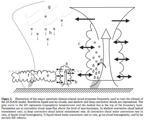
From Mauritsen et al 2012
Figure 3
And how changing some of these parameters affects (over a short run) “headline” parameters like TOA imbalance and cloud cover:
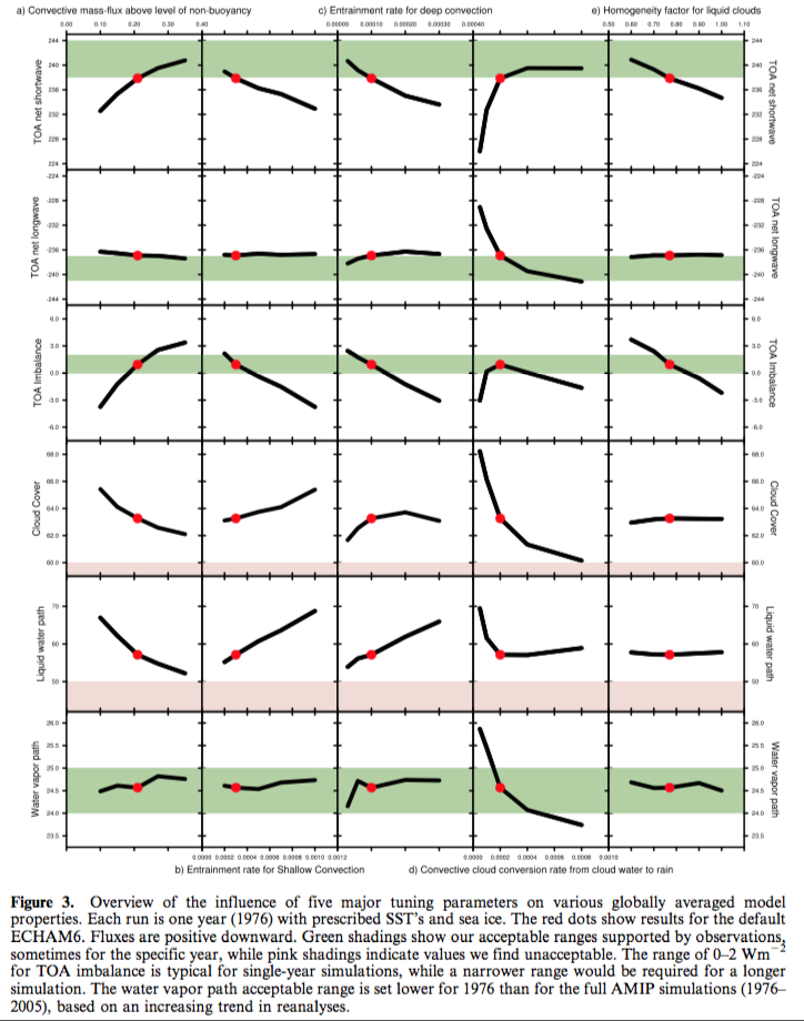
From Mauritsen et al 2012
Figure 4 – Click to Enlarge
There’s also quite a bit in the paper about tuning the Arctic sea ice that will be of interest for Arctic sea ice enthusiasts.
In some of the final steps we get a great insight into how the whole machine goes through its final tune up:
..After these changes were introduced, the first parameter change was a reduction in two non-dimensional parameters controlling the strength of orographic wave drag from 0.7 to 0.5.
This greatly reduced the low zonal mean wind- and sea-level pressure biases in the Northern Hemisphere in atmosphere-only simulations, and further had a positive impact on the global to Arctic temperature gradient and made the distribution of Arctic sea-ice far more realistic when run in coupled mode.
In a second step the conversion rate of cloud water to rain in convective clouds was doubled from 1×10⁻⁴ s-1 to 2×10⁻⁴ s-1 in order to raise the OLR to be closer to the CERES satellite estimates.
At this point it was clear that the new coupled model was too warm compared to our target pre- industrial temperature. Different measures using the convection entrainment rates, convection overshooting fraction and the cloud homogeneity factors were tested to reduce the global mean temperature.
In the end, it was decided to use primarily an increased homogeneity factor for liquid clouds from 0.70 to 0.77 combined with a slight reduction of the convective overshooting fraction from 0.22 to 0.21, thereby making low-level clouds more reflective to reduce the surface temperature bias. Now the global mean temperature was sufficiently close to our target value and drift was very weak. At this point we decided to increase the Arctic sea ice volume from 18×1012 m3 to 22×1012 m3 by raising the cfreeze parameter from 1/2 to 2/3. ECHAM5/MPIOM had this parameter set to 4/5. These three final parameter settings were done while running the model in coupled mode.
Some of the paper’s results (not shown here) are some “parallel worlds” with different parameters. In essence, while working through the model development phase they took a lot of notes of what they did, what they changed, and at the end they went back and created some alternatives from some of their earlier choices. The parameter choices along with a set of resulting climate properties are shown in their table 10.
Some summary statements:
Parameter tuning is the last step in the climate model development cycle, and invariably involves making sequences of choices that influence the behavior of the model. Some of the behavioral changes are desirable, and even targeted, but others may be a side effect of the tuning. The choices we make naturally depend on our preconceptions, preferences and objectives. We choose to tune our model because the alternatives – to either drift away from the known climate state, or to introduce flux-corrections – are less attractive. Within the foreseeable future climate model tuning will continue to be necessary as the prospects of constraining the relevant unresolved processes with sufficient precision are not good.
Climate model tuning has developed well beyond just controlling global mean temperature drift. Today, we tune several aspects of the models, including the extratropical wind- and pressure fields, sea-ice volume and to some extent cloud-field properties. By doing so we clearly run the risk of building the models’ performance upon compensating errors, and the practice of tuning is partly masking these structural errors. As one continues to evaluate the models, sooner or later these compensating errors will become apparent, but the errors may prove tedious to rectify without jeopardizing other aspects of the model that have been adjusted to them.
Climate models ability to simulate the 20th century temperature increase with fidelity has become something of a show-stopper as a model unable to reproduce the 20th century would probably not see publication, and as such it has effectively lost its purpose as a model quality measure. Most other observational datasets sooner or later meet the same destiny, at least beyond the first time they are applied for model evaluation. That is not to say that climate models can be readily adapted to fit any dataset, but once aware of the data we will compare with model output and invariably make decisions in the model development on the basis of the results. Rather, our confidence in the results provided by climate models is gained through the development of a fundamental physical understanding of the basic processes that create climate change. More than a century ago it was first realized that increasing the atmospheric CO2 concentration leads to surface warming, and today the underlying physics and feedback mechanisms are reasonably understood (while quantitative uncertainty in climate sensitivity is still large). Coupled climate models are just one of the tools applied in gaining this understanding..
[Emphasis added].
..In this paper we have attempted to illustrate the tuning process, as it is being done currently at our institute. Our hope is to thereby help de-mystify the practice, and to demonstrate what can and cannot be achieved. The impacts of the alternative tunings presented were smaller than we thought they would be in advance of this study, which in many ways is reassuring. We must emphasize that our paper presents only a small glimpse at the actual development and evaluation involved in preparing a comprehensive coupled climate model – a process that continues to evolve as new datasets emerge, model parameterizations improve, additional computational resources become available, as our interests, perceptions and objectives shift, and as we learn more about our model and the climate system itself.
Note 1: The link to the paper gives the html version. From there you can click the “Get pdf” link and it seems to come up ok – no paywall. If not try the link to the draft paper (but the formatting makes it not so readable)


Thanks for this fascinating post.
“Within the foreseeable future climate model tuning will continue to be necessary as the prospects of constraining the relevant unresolved processes with sufficient precision are not good.”
This is something that is rarely admitted in public. If you look at Fig 10.5 in AR5 Plot d) shows the total forcing for each model instance in the ensemble. They are ALL different. So this implies that each model has used slightly different net values for anthropogenic forcing, and for natural forcings in order to match the past 20th century warming.
Clive,
Have you read Jeffrey Kiehl’s 2007 paper: Twentieth century climate model response and climate sensitivity?
Worth a read as it addresses this very question.
[…] der Webseite „Science of DOOM“ bin ich auf einen Artikel von Mauritsen et al. gestoßen über das […]
Your link to the paper is paywalled. http://www.mpimet.mpg.de/fileadmin/staff/klockedaniel/Mauritsen_tuning_6.pdf appears to be a free copy.
Minor quibble: re absolute vs anomalies, I think you should point out that the absolute value isn’t known from obs, to within an accuracy that I can’t remember.
William,
Thanks. It seems that the paper is actually free, even in published form, but you have to go to the html overview page and click “Get pdf”.
I updated the article.
William,
I’m not following, unless you are saying every measurement has an error associated?
I was commenting on your “It was interesting to see that if we plot the “actual modeled temperatures” from 1850 to present the picture doesn’t look so good”. I thought you were saying that the models, when looking at the absolute temperatures rather than the anomalies, appear more spread, and further from the observations. But the observations themselves, as an absolute, are more uncertain.
Looking again, I’m now somewhat puzzled, as the paper says “Figure 1. Absolute temperatures from climate model historical realizations and future scenarios. Black line is the HadCRUT3v blended land and ocean temperature dataset and red line is CRUTEM3v land-only temperatures [Brohan et al., 2006]”. I thought the CRU stuff was always given as anomalies.
The CRU station data are given as absolute monthly temperatures. You certainly can calculate the average monthly global temperature. This is what you get. To calculate the “anomaly” CRU use monthly averaged temperatures calculated at each station between 1961 and 1990. The station anomaly is then derived as the measured temperature minus one of the relevant 12 average values. These anomalies are then area averaged over each hemisphere to give the usual graph using exactly the same algorithm as for temperature.
The argument to use anomalies instead of absolute temperatures is simply that it averages out seasonal variations and hides biases in the distribution of stations especially in the early period when most stations were located in Europe and North America.
A significant uncertainty may be related to the definition of the temperature in the sense that the model cannot calculate specifically temperatures that correspond to the way the measurements are done (like air temperature at the altitude of 2 m in land areas and temperature of the water near surface measured using specific methods. Relating such temperatures to either the surface or to the near surface cells introduces surely uncertainty that exceeds probably significantly the uncertainties in determining the anomaly. (Most of these factors cancel fully in the anomaly).
Whenever aggregated models are used in any field, some problems occur in relating model variables to observed variables. What’s superficially the same variable, may differ significantly when looked at more carefully.
The observations in say 1900 can’t have that much uncertainty. We know present day temperature? So unless we are unsure whether the world has warmed over the last 114 years..
I’m sure there should be error bars on the observations but I have no idea what they are. +/-0.5’C? That seems too high. But even with that, the modeled absolute temperatures have a much greater range.
It seems, as the paper makes clear, that what you choose as a target is what gets accomplished, and certain targets are necessary to get your model over the line.
Last 150 year temperature anomaly history is a must, therefore, anomalies are good.
If last 150 year absolute temperature history was a must we would see a much tighter range in figure 1.
When I emphasized difficulties in linking observed absolute temperatures to the model temperature variables, it might have been good to point out that weather models (and probably also reanalyses that take advantage of weather models) are certainly helpful in closing the gap. How much uncertainty is left in the relationship, I really don’t know.
Assuming that the issue is looked at carefully it should not be too difficult to get closer than 0.5C for areal coverage like that of HadCRUT4. Including polar regions might add significantly to the uncertainty.
Pekka,
Weather models don’t have to worry about drift. They can start with the right surface temperature – in fact they do, they get their starting point from current observations via reanalysis products.
So one year with TOA radiation balance out by 5W/m2 is not going to be a problem in a weather model. It doesn’t have to calculate the right surface temperature from model parameters.
SoD,
I referred to the weather models only as a tool for linking the model variables of climate models to the real world. A weather model is detailed enough for a reasonably precise connection between what’s a surface temperature in the model and what are the real world values that have been measured.
In a model of large grid cells and complex parametrizations for subgrid level physics the automatic connection is very imprecise. With coniderable extra effort it’s possible to figure out, how the temperatures of the model grid relate to the air temperature 2 m from surface and the temperature of the ocean water just below the surface. As long as climate models are used to describe anomalies this extra analysis may be left totally undone. In that case the absolute values obtained from the models cannot really be compared with observed data with acceptable accuracy.
The differences in absolute temperatures obtained from different climate models may also be, in part, due to different implied definitions of surface temperature.
> the model cannot calculate specifically temperatures that correspond to the way the measurements are done (like air temperature at the altitude of 2 m in land areas…
That’s another point. But its not totally true: the Hadley models certainly *do* (attempt to) calculate a 2m temperature, based on the std surface layer parametrisations.
> +/-0.5′C? That seems too high. But even with that, the modeled absolute temperatures have a much greater range
Yes, I agree with that.
A related question is:
Do the models agree better on the absolute temperature of the upper troposphere?
AOGCMs do not predict current and historical temperatures to within +/-0.5 degC. They predict temperature change (ie, temperature anomalies) more precisely and most projections are made in terms of temperature change or temperature anomaly, which ignores the discrepancies in absolute temperature.
From: http://judithcurry.com/2013/07/09/climate-model-tuning/
It’s useful to see what the IPCC third assessment report said about models (p.476 onwards):
[Emphasis added].
There’s no doubt that models have come a long way. We have much better observations. Lots of work has taken place. Observational constraints on specific parts of the model and inter-comparison work has allowed lots of improvements to individual components.
If you know the value you need to get to, you can make good progress, you can test your result against a target.
The problem, nicely outlined by this paper, is that there is no tight physical constraint on any one of 10s of parameters. Just on the result that pops out.
Flux adjustments have also been used to study some more specific issues. The paper of Kosaka and Xie is an example of that. They made a rather strong time dependent local flux adjustment to force the temperature of the eastern equatorial pacific to the observed value over the period 1970-2012.
It would be interesting to understand how much of the tuning needed in parameters is because of the inability to model at fine mesh sizes or even to use variably-sized meshes. Maybe it’s not known, but, certainly, if the same grid sizes would be worthless simulating oceans or currents. And there was a dramatic demonstration in the past couple of years of how much better ice flow-in-basin modes were if fine or variably-sized mesh models were used for them.
Related to the computational question is the computing facilities available for running the models, and whether there exist bigger ones that could be applied. If they are not applied, it would be interesting to know why not. I know there is a severe shortage of people skilled at describing, programming up, and running these models.
Regarding the quote from the paper “Climate models ability to simulate the 20th century temperature increase with fidelity has become something of a show-stopper as a model unable to reproduce the 20th century would probably not see publication, and as such it has effectively lost its purpose as a model quality measure” in paragraph 66, while I am no climate modeler, it seems to me this is a mistake, however well-intentioned it might be. It is entirely possible that there is an overall consistent explanation for a dataset which does not explain a subset particularly well. That can be because of simplifications in the model, or it can be because there’s something odd about the data in that subset, or it can be because that data is somehow just recorded or measured incorrectly. If the likelihood value for those data given the best estimated parameters and the best understood and performing model is low, so be it, it’s low.
Worse, I note the comment is that the observational values do not produce a stable model, not one which says those values are impossible. This suggests there are dynamics peculiar to the numerical coupling within the model itself which are not stable, and these may not be any evidence of disagreement with observations at all.
I think those models have problems with grid size because the parameterizations can’t handle the “small scale” phenomena, the grid is too coarse to describe the static description, and the feedbacks are probably not as depicted. All of these problems can be gradually resolved over the years, but it takes time and money.
SoD,
Thanks for an informative post. It is interesting that the ensemble is biased cool relative to observations. A cool bias would appear to lower evaporation rates and so reduce tropospheric convection and cloud formation. Do you know if there is any correlation between a model’s absolute bias (relative to surface temperature observations) and that model’s diagnosed sensitivity?
stevefitzpatrick,
That’s a good point that the authors also comment on:
The paper has a brief look at the topic of sensitivity. Here’s how they introduce it:
And so they show their figure 4 (my figure 2), which shows the slope of temperature drift due vs out of balance TOA for many models. They have put two slopes on the figure, you can see that most models drift along the “4.5K for doubling CO2” slope.
SoD,
Yes, I noted that the slope of the drift (your fig 2) was related to the model’s diagnosed sensitivity. But since the modelers work to get near zero drift, this seems a very limited way to evaluate possible correlation between a model’s absolute temperature bias and that same model’s sensitivity. The CIMP5 models in figure 2 appear to all have near zero drift. AR5 (chapter 8 I think) includes a list of sensitivity values for ~ 20-25 models (I can’t remember the exact number). If the absolute temperature bias for those same models is available, then any correlation would be easy to see. I just don’t know where to find the absolute bias for each model. Do you?
stevefitzpatrick,
I’m a novice when it comes to the details of getting hold of model outputs.
But I did find a graph further on in chapter 9 of AR5 (p.817) which might be what you are looking for:
SoD,
Exactly what I was looking for, thanks.
The diagnosed sensitivity does seem to be inversely correlated with absolute temperature (higher sensitivity with lower absolute temperature), though there is clearly a lot of scatter.
This paper: “Analysis of the Model Climate Sensitivity Spread Forced by Mean Sea Surface Temperature Biases”,
suggests that model average SST can have a big influence on sensitivity.
SoD,
I hand digitized the IPCC AR5 graphic (as best I could, I don’t claim perfect accuracy) for the 1961 to 1990 data. The regression of model sensitivity against absolute model temperature yields a slope of about -0.45 +/- 0.29 C (one sigma) in equilibrium climate sensitivity for each degree increase in model absolute temperature. The r^2 is only ~0.11, and the F-statistic is ~2.6 with 20 degrees of freedom. This corresponds, if I read the table correctly, to a chance of ~15% that the correlation is in fact spurious (~85% chance that the correlation is real). This is not strong evidence, but it does at least suggest some correlation between sensitivity and absolute model temperature.
stevefitzpatrick,
The low r2 I believe – we can see that from the graph.
Your comment is a convenient “peg” for me to hang my question on..
To me, statistical significance in these cases just has zero meaning. These are not independent “events”.
I hope someone can enlighten me about how to “do statistics” on “calculations done by different sets of people who read each other’s papers, share ideas at conferences, copy parameterizations and run similar models”.
I can understand the statistics of the example I showed in Ensemble Forecasting because there we are saying, if (and only if) we have uncertainty in initial conditions as identified, and uncertainty in the parameterization as identified, then the mean, spread, standard deviation of results all have some meaning. They express the uncertainty in the final result, based on our uncertainty of some conditions.
But if I write a model of convective flow, pick some parameters that seem to make it work how we expect, and you write a model of convective flow with a similar starting point but a few different assumptions, and so do 18 other people – what can we say about our 20 different results?
I think we can look at them and try and understand where the differences come from. We can see that there’s a bit of trend in one direction or another. And we can pick apart the reasons behind differences and similarities and hopefully figure out how to improve models.
But “statistical significance” and “probability”?
SoD,
“I think we can look at them and try and understand where the differences come from. We can see that there’s a bit of trend in one direction or another. And we can pick apart the reasons behind differences and similarities and hopefully figure out how to improve models.”
Sure, but if there is a correlation between absolute temperature bias and model sensitivity, that is a good starting point to try to gain a better understanding. It may mean nothing, but it may also be a hint of something more interesting, like how errors in water vapor pressure tilt the diagnosed sensitivity one way or another. Or how cloud formation and cloud radiative forcing is linked to absolute temperatures (as opposed to anomalies). I don’t think it hurts to consider the possibility of useful information contained in this sort of correlation. You seem to object to a statistical analysis; but it is not clear to me why. Had that analysis shown 95% or 99% in an F test would it still be objectionable?
stevefitzpatrick,
Object is the wrong word. I’m looking for insight. Often my questions tend to come over somewhat adversarial, which I don’t intend.
What does the statistical significance / probability mean?
If I believe the dice is unbiased, throw it 10 times and get ‘6’ 7 times, ‘5’ 2 times and ‘4’ once I can work out the likelihood that the dice is unbiased. The probability tells me something about the dice. If I do the same test 1000 times and really do have an unbiased dice I can give some advance expectation of the number of times we would expect to get that kind of high score over 10 throws. The probability gives me useful information. Probability theory is useful.
What does “85% chance that the correlation is real” tell you? The calculation of probability – as far as I understand it – is based on the notion that each is some independent test.
I agree with looking at the correlations we can see in the scatter graph and using the relationships to think about what we should investigate – no argument with that. Plotting things out and looking at the results is definitely the way to go.
I’m 100% sure that the correlation between the ECS and GMSAT is low and I’m 100% sure that there is a slight negative correlation.
Where does chance and probability come in?
I think you are saying it is 85% certain that this negative correlation is not a chance result. And if you are saying that I have no idea what it means. Alternatively, I suspect that the calculation of 85% has no validity.
Possibly I would fail all statistics courses even though I think I understand the basis behind probability theory.
The line would either be really obvious with 20 points, or there would be 200 points on the graph. If the line was more obvious with 20 points no one would be concerned about the probability because we would all see the obvious relationship. If there was the same scatter diagram with 200 points providing the 95 or 99% probability then I would have the exact same question.
And you don’t have to defend your statement if this line of questioning is frustrating. Like I say, I’m looking for insight.
Looking at the IPCC Figure 9.42a we can make one observation: The upper right-hand corner is empty. Adding two models (2 points from each) to that corner would remove the effect – and surely also the weak correlation observed. If the expectation value is 2, Poisson distribution gives the probability of 0.135 for zero. Thus this is not statistically significant assuming independence of the values.
Looking at the trend is not really meaningful, but we might ask, whether there is a reason for the empty upper right corner. Is that just accidental, or is there some other reason like a difficulty in building a plausible enough model that goes there, or something else that has led the modelers to search elsewhere. The modelers themselves might be able to tell the reason, if the situation is not accidental.
We have learned that most of the models have a cold bias at the surface. I have made some comments related to that and continue by reformulating, what I have in mind.
The surface may be too cold for two reasons:
– The whole troposphere is too cold
or
– The parametrization that links the surface temperature to the atmospheric temperatures is wrong. In other words the lapse rate is too low at least at some altitudes or the surface is too cold relative to the average temperature of the lowest atmospheric cell.
If the models are tuned to maintain the energy balance at TOA with a correct value of the albedo, the second alternative must be closer to the truth as far as I understand. A high value for the albedo is expected to lead to the first alternative.
Further question may be presented on the errors a too cold surface creates. The most obvious issue is evaporation, but that could be compensated by adjusting the parametrization of the evaporation rate.
SoD,
The only way I know to test if a weak correlation is likely real is to apply a statistical test. You say you are 100% sure there is a slight negative correlation. But how can you know if that arises only by chance, as opposed to causally, unless you do some kind of statistical test?
Pekka,
That any model is biased quite low relative to measurements suggests to me one or more obvious errors, so I am a little surprised by that. I mean, measured mean surface temperature does have some associated uncertainty range, but when a model is well outside that range, I would expect the modelers to stop right there and try to figure out why. Surface temperature seems to me to be a key variable, because it influences the vapor pressure of water and the rate of ice melt/formation, so I don’t at all understand why modelers would not adjust the model to reasonably match the measured temperature; I would have guessed this to be a very important constraint, but it apparently it is not.
My understanding is that all models have tropospheric temperatures tightly linked to surface temperature, at least over the tropical ocean. So an error of a single degree at the surface would likely influence the entire troposphere’s temperature and the lapse rate profile.
stevefitzpatrick
These ‘events’ are not ‘independent’ of each other.
There is no statistical test that is justifiable here – my hypothesis, for discussion.
‘By chance’ is meaningless in this context. There is just a weak correlation. That’s all we can say.
One day I will think of a suitable analogy.
SoD,
OK. Suppose that there are several different parameters which, singly and jointly, influence the accuracy of the models’ surface temperature, as well as multiple other model characteristics. Further suppose that each modeling group selects a different combination parameter values based on their different experiences, prejudices, beliefs, and hunches, as well as which model behaviors they think are the most important to match observations.
Under these circumstances, it seems to me that there are (perhaps) sufficient permutations and combinations of parameter values that each model’s absolute surface temperature is at least to a degree independent of other models, and that each model represents a more-or-less randomly selected surface temperature, taken from a theoretically large population of all the possible combinations of model parameters. In this case statistical tests may be reasonable to try.
I think a more important question is if the (weak) correlation is caused by differences in surface temperature, or if the model parameters which influence surface temperature just happen to also influence the model’s sensitivity. IOW, correlation or causation.
stevefitzpatrick,
Under your restrictive conditions this becomes a random selection from an infinite set of parameters. In this case, probability theory is useful and your “probability that this is a spurious result” is a useful piece of additional information to the relationships we can see on the scatter diagram.
I believe the real world of climate modeling is completely different from this. They read each others’ papers, meet at conferences, work on the CMIP5 model inter-comparison project, learn from each others parameter/model problems and share the same set of preconceptions.
I consider myself a skeptic, but I don’t mind exchanging ideas with you guys. My professional experience running complex models goes back to the early 1980’s using “3d dynamic compositional” oilfield reservoir models. I won’t go into the advances made in the last 30 years, but as you can imagine the models have improved a lot.
If you are interested, you may wish to read this item about an interesting approach developed over the last 10 years (more or less), which we call the top down approach.
Click to access mohaghegh2.pdf
I can’t get into some of the techniques we use because some are considered confidential, but I can give you a hint, a top down approach can be used to tune the classic 3d grid model, and this includes tuning parameterization. If you have enough computer horsepower you can also run multiple realizations (I worked in a shop where the customary number of realizations in an ensemble was set at 50). However I have read you do seem to run short on processing power when compared to the overall needs. However, maybe you could try forming a consortium to run a project to experiment with improved tuning methods.
Hope this helps, and do remember I’m trying to be helpful. I got the sense you do have a handicap because the models are so large and complex, and the data set to be matched is incomplete.
The problem with your Figure 4 (called Figure 3 in the paper) is that we are looking at the change in one parameter when the other parameters are all held fixed. Parameter d) has an optimum value shown by the red dot, but only when the other four parameters are at their red dots (and other parameters are also fixed). Work with perturbed physics ensembles (where all parameters are varied at random) suggests that other optimum sets of these five parameters might be found if a more comprehensive search were computationally feasible. Instead of a single clear optimum, one finds a multi-dimensional surface with multiple local optima and no clear direction to a global optimum – assuming such an optimum even exists. Perhaps I’m exaggerating the extent of this problem. Climate sensitivity varies significantly with the choice of parameters. See:
Click to access nature_first_results.pdf
Click to access sanderson08jc.pdf
From the first paper: “Can we coherently predict the model’s response to multiple parameter perturbations from a small number of simulations each of which perturbs only a single parameter? The question is important because it bears on the applicability of linear optimization methods in the design and analysis of smaller ensembles. Figure 2c shows that assuming that changes in the climate feedback parameter combine linearly provides some insight, but fails in two important respects. First, combining uncertainties gives large fractional uncertainties for small predicted and hence large uncertainties for high sensitivities. This effect becomes more pronounced the greater the number of parameters perturbed. Second, this method systematically underestimates the simulated sensitivity, as shown in Fig. 2c, and consequently artificially reduces the implied likelihood of a high response. Furthermore, more than 20% of the linear predictions are more than two standard errors from the simulated sensitivities. Thus, comprehensive multiple-perturbed-parameter ensembles appear to be necessary for robust probabilistic analyses.”
“From the second: “Requiring models to match all observations simulta- neously proved a more difficult task for all of the ensembles. The ANN simulated ensemble suggested that model parameters could at best be tuned to a compro- mise configuration with a finite error from the obser- vations. This “best model discrepancy” was found to increase with the inclusion of increasing numbers of separate observations, and was not itself a strong function of S [climate sensitivity]. Hence although models can be found to independently reproduce seasonal differences in the three observation types, there is no single model that can reproduce all three simultaneously. The relative errors of best models at different sensitivities will decrease and the irreducible error of the best-performing model increases dramatically as more observations are added. Thus the “all fields” approach yields no models that are fully consistent with observations, although it shows a minimum in error at S = 4 K.
Such an effect is a natural by-product of tuning an imperfect model to match observations: it is easy to tune parameters to match a single observation, but impossible to match all simultaneously. Such an effect must be considered in predictions of sensitivity such as Knutti et al. (2006) and Piani et al. (2005), where trends determined through analysis of an imperfect ensemble were applied directly to observations. We have found that the perfect model state may be unattainable through parameter perturbations alone, hence an estimation of irreducible error should be included when using ensemble-trained predictors of S.”
All papers and presentations from the group that did this work are freely available at: http://www.climateprediction.net/publications/
Frank,
Your first example, Uncertainty in predictions of the climate response to rising levels of greenhouse gases, Stainforth et al, Nature (2005) is an interesting paper.
Here’s the spread of results from 2000 simulations with different parameters under the scenario of doubling CO2 (circled area), note the frequency colorbar:
I also highlight part of the quote you cited:
Another important part of this paper deserves attention.
The models – for the aim of getting more parameter space explored with the computing power available – used a “mixed layer ocean”. This means the ocean is not “real”. It’s something like a 50m depth with no deep ocean currents, nowhere for cold water to sink to.
This introduces some problems. One problem is that some of the ensemble members cooled significantly – you can see it in the middle section of the top graph.
Here’s the authors in the Supplementary Information (Nature papers are too short):
So these models were removed from the results.
There is nothing wrong with this – we remove an obvious unphysical model, once we have understood the “failure mechanism”.
But it demonstrates that a model with a “mixed-layer ocean” is itself not a very good model, or at least, has a severe limitation. Perhaps a significant proportion of the results are actually unphysical but in a less obvious way.
When we know the right answer it is easy to remove the bad results.
SOD: I was hoping that you were way ahead of me (as usual) and planning to discuss perturbed physics ensembles, especially newer stuff I haven’t read. Stainforth and colleagues got their first paper published in Nature by pointing out that there could be many viable climate models with much higher ECS than those used by the IPCC. But I think it really says that the range of the output from climate models used by the IPCC doesn’t come to describing the range of possible climate futures that are consistent with known physics. So I’ve latched onto the term “ensemble of opportunity” to describe the IPCC models.
You are certainly correct that compromises in the model (the slab ocean, others?) in order to make computation practical. Perhaps tuning works better with more sophisticated models than the ones used here.
When looking for the Supplementary Information for Stainforth et al 2005 on the Nature site, I found a short review article: Towards objective probabalistic climate forecasting, Allen & Stainforth, Nature (2002):
[Emphasis added].
Thanks SoD
I note you didn’t put a pithy “conclusion” section to this post stating what you think might be the take home messages here. So what exactly can we say from all this? I know if you say something with any conviction in climate science then somebody will jump all over you but if we take one of the highlighted quotes
“Climate models ability to simulate the 20th century temperature increase with fidelity has become something of a show-stopper as a model unable to reproduce the 20th century would probably not see publication, and as such it has effectively lost its purpose as a model quality measure.”
Does this mean if somebody says “look how well the models reproduces the 20th century GMT anomaly” as a defense for the skill of climate models then it’s actually reasonable to be skeptical of what that actually tells us? Should it make somebody question exactly what the projection part of the simulation tell us? It seems like a skeptics wet-dream!
HR,
Well spotted. I don’t have a Conclusion in this article because I mostly cited from the paper. In Ensemble Forecasting I didn’t have a “Conclusion”, instead a “Discussion” because I wasn’t sure what to conclude.
And as you note, the paper didn’t hide its takeaway message.
It seems reasonable to be skeptical of the “apparent skill” in climate models.
That is, by reproducing the last 150 years of temperature anomaly, climate models have not necessarily demonstrated they have any predictive skill.
That said, there are lots of papers on climate models decadal skill that I haven’t read. Perhaps there is plenty of evidence. I haven’t focused on GCMs in my reading. I have gathered up a few papers after reading this one..
I believe I’ve said this before. Reproducing the last 150 years of the global temperature anomaly is a necessary but not sufficient condition for demonstrating predictive skill. Skill at reproducing regional anomalies for the same period would be nice too, but hasn’t happened as far as I know.
Perhaps one approach is like that for fitting parameters to a sample distribution.
To avoid overfitting you take half the sample and fit – then see how it works for the whole sample. That hilarious paper by the forestry guys, Nikolov and Zeller, is a great example of how not to do it (as well as not understanding anything about atmospheric physics etc etc).
So applying that broad concept to climate, the modeling team works hard to produce a climate simulation to recreate:
– absolute temp
– temp anomalies
– TOA balance
– precipitation
But they don’t get to see any data on the MOC, arctic ice and some other key parameters.
The skill of the model is then determined by their ability to model the unseen parameters, not their ability to model the parameters they targeted.
Just a thought. Probably everyone in climate modeling is doing this already..
Splitting the data in parts and fitting to one part may tell something, but the fundamental problem is that all date known during the model development and tuning may have influenced the model in some way. Therefore statistical tests that satisfy all formal requirements are possible only using new data that tells something totally unknown previously.
Tests that are done violating the requirement of independence may tell a lot, but it’s very difficult (or impossible) to tell, how powerful such tests are.
SOD: I think you’ve got an interesting idea: tune your parameters using some observations and test the resulting model against other observations of current climate. Then tune using a different set of observations and test a different set of withheld data. You’d probably want to always tune using observed values for TOA OLR and SWR because these are critical to the planetary energy balance. Maybe you’ll converge on the same set of parameters. Maybe you’ll learn there are multiple local optima that perform about as well as each other. (Something this sensible has probably been tried.)
DeWitt Payne wrote: on July 16, 2014 at 11:13 pm
“I believe I’ve said this before. Reproducing the last 150 years of the global temperature anomaly is a necessary but not sufficient condition for demonstrating predictive skill. Skill at reproducing regional anomalies for the same period would be nice too, but hasn’t happened as far as I know.”
How accurately do we have to reproduce the last 150 years of the global temperature anomaly? Are the peak around 1940 and the current pause noise or are these unforced variability. You can assess the role of natural variability only with the assistance of a model, but you want to judge the adequacy of a model by its ability to reproduce a historical record that contains both forced and unforced variability. This is an inherently circular argument. If you believe Nic Lewis, it appears as if a desire to “explain” the flat temperatures around 1960 with rising aerosols has probably led to models which are too sensitive to aerosols.
I believe you must also get the absolute temperature, not the anomaly, correct. If not, your boundaries between frozen and liquid water will be wrong or set by compensating errors.
If you haven’t read Lorenz (1991), “Chaos, Spontaneous Climatic Variability and the Detection of the Greenhouse Effect”, it would be worth your time. The article was written by a far-seeing expert before the world was investing perhaps a billion(?) dollars per year and thousands(?) of careers in GCMs and relying on them to tell us what we needed to do with the enerby sector of trillion dollar economies
I asked the lead author of the paper, Thorsten Mauritsen, about the idea above:
His answer is very interesting:
He also added:
I just read a new GRL paper, Evaluating climate model performance in the tropics with retrievals of water isotopic composition from Aura TES, Robert D. Field et al (2014). One of the coauthors is the famous Gavin Schmidt.
Interesting that they cited Mauritsen et al 2012 (the subject of this article).
The paper is about using water isotopes (HDO vs H2O) that are now measured by the Aura Tropospheric Emission Spectrometer (TES) and comparing the ratios to values in models. The fractionation process is quite simple compared with convection and condensation/evaporation/precipitation processes, so it can be used to put better constraints on models and highlight problem areas.
A little more detail:
They didn’t comment on what happened to TOA radiation balance from the model changes. Note that the model is an AGCM (atmospheric GCM) running from SST observations, not a “fully-coupled” AOGCM (atmosphere-ocean-GCM).
Here is the overall model performance vs observations. Top graph is “observation” in the mid-upper troposphere, 2nd graph is the model that went into IPCC AR5 and the 3rd graph is that model after all perturbation changes (called AR5′):
And here is the δD – the isotopic composition of water vapor in observation and models:
[…] the idea of much larger ensembles of climate models. The Stainforth paper was discussed in the comments of Models, On – and Off – the Catwalk – Part Four – Tuning & the Magic Behind […]
Kenneth Fritsch has been doing some work on calculating TCR and ECS from the CMIP5 models over at The Blackboard (see comments starting here). It turns out that you have to subtract the TOA imbalance in the pre-industrial control period (PIC) to get the same values as reported in the literature. I find this to be very disturbing. Apparently all TOA imbalances are not equal. Oh, you can hand wave that it’s the slow ocean response that’s the problem, but a 3 W/m² TOA imbalance should have the same transient effect whether it’s from a 4XCO2 spike or during the model spin-up.
The slow equilibration of the models is exactly why the ECS is so much larger than the TCR. It’s not at all clear that this is true in the real world.
[…] larger ensembles of coarser resolution climate models, and was discussed in the comments of Models, On – and Off – the Catwalk – Part Four – Tuning & the Magic Behind […]
[…] Part Four of this series we looked at the paper by Mauritsen et al (2012). Isaac Held has a very interesting […]
[…] on temperature anomaly actually do quite badly on the actual surface temperature. See Models, On – and Off – the Catwalk – Part Four – Tuning & the Magic Behind the Scenes – you can see that many “fit for purpose” models have current climate halfway to […]
[…] Five – More on Tuning & the Magic Behind the Scenes and also in the earlier Part Four we looked at the challenge of selecting parameters in climate models. A recent 2017 paper on this […]
[…] Mauritsen who was the lead author of Tuning the Climate of a Global Model, looked at in another old article, and another co-author is Jean-Christophe Golaz, lead author of the paper we looked at […]