[I started writing this some time ago and got side-tracked, initially because aerosol interaction in clouds and rainfall is quite fascinating with lots of current research and then because there are many papers on higher resolution simulations of convection that also looked interesting.. so decided to post it less than complete because it will be some time before I can put together a more complete article..]
In Part Four of this series we looked at the paper by Mauritsen et al (2012). Isaac Held has a very interesting post on his blog – and people interested in understanding climate science will benefit from reading his blog – he has been in the field writing papers for 40 years). He highlighted this paper: Cloud tuning in a coupled climate model: Impact on 20th century warming, Jean-Christophe Golaz, Larry W. Horowitz, and Hiram Levy II, GRL (2013).
Their paper has many similarities to Mauritsen et al (2013). Here are some of their comments:
Climate models incorporate a number of adjustable parameters in their cloud formulations. They arise from uncertainties in cloud processes. These parameters are tuned to achieve a desired radiation balance and to best reproduce the observed climate. A given radiation balance can be achieved by multiple combinations of parameters. We investigate the impact of cloud tuning in the CMIP5 GFDL CM3 coupled climate model by constructing two alternate configurations.
They achieve the desired radiation balance using different, but plausible, combinations of parameters. The present-day climate is nearly indistinguishable among all configurations.
However, the magnitude of the aerosol indirect effects differs by as much as 1.2 W/m², resulting in significantly different temperature evolution over the 20th century..
..Uncertainties that arise from interactions between aerosols and clouds have received considerable attention due to their potential to offset a portion of the warming from greenhouse gases. These interactions are usually categorized into first indirect effect (“cloud albedo effect”; Twomey [1974]) and second indirect effect (“cloud lifetime effect”; Albrecht [1989]).
Modeling studies have shown large spreads in the magnitudes of these effects [e.g., Quaas et al., 2009]. CM3 [Donner et al., 2011] is the first Geophysical Fluid Dynamics Laboratory (GFDL) coupled climate model to represent indirect effects.
As in other models, the representation in CM3 is fraught with uncertainties. In particular, adjustable cloud parameters used for the purpose of tuning the model radiation can also have a significant impact on aerosol effects [Golaz et al., 2011]. We extend this previous study by specifically investigating the impact that cloud tuning choices in CM3 have on the simulated 20th century warming.
What did they do?
They adjusted the “autoconversion threshold radius”, which controls when water droplets turn into rain.
Autoconversion converts cloud water to rain. The conversion occurs once the mean cloud droplet radius exceeds rthresh. Larger rthresh delays the formation of rain and increases cloudiness.
The default in CM3 was 8.2 μm. They selected alternate values from other GFDL models: 6.0 μm (CM3w) and 10.6 μm (CM3c). Of course, they have to then adjust others parameters to achieve radiation balance – the “erosion time” (lateral mixing effect reducing water in clouds) which they note is poorly constrained (that is, we don’t have some external knowledge of the correct value for this parameter) and the “velocity variance” which affects how quickly water vapor condenses out onto aerosols.
Here is the time evolution in the three models (and also observations):
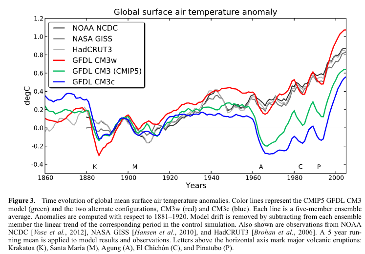
From Golaz et al 2013
Figure 1 – Click to enlarge
In terms of present day climatology, the three variants are very close, but in terms of 20th century warming two variants are very different and only CM3w is close to observations.
Here is their conclusion, well worth studying. I reproduce it in full:
CM3w predicts the most realistic 20th century warming. However, this is achieved with a small and less desirable threshold radius of 6.0 μm for the onset of precipitation.
Conversely, CM3c uses a more desirable value of 10.6 μm but produces a very unrealistic 20th century temperature evolution. This might indicate the presence of compensating model errors. Recent advances in the use of satellite observations to evaluate warm rain processes [Suzuki et al., 2011; Wang et al., 2012] might help understand the nature of these compensating errors.
CM3 was not explicitly tuned to match the 20th temperature record.
However, our findings indicate that uncertainties in cloud processes permit a large range of solutions for the predicted warming. We do not believe this to be a peculiarity of the CM3 model.
Indeed, numerous previous studies have documented a strong sensitivity of the radiative forcing from aerosol indirect effects to details of warm rain cloud processes [e.g., Rotstayn, 2000; Menon et al., 2002; Posselt and Lohmann, 2009; Wang et al., 2012].
Furthermore, in order to predict a realistic evolution of the 20th century, models must balance radiative forcing and climate sensitivity, resulting in a well-documented inverse correlation between forcing and sensitivity [Schwartz et al., 2007; Kiehl, 2007; Andrews et al., 2012].
This inverse correlation is consistent with an intercomparison-driven model selection process in which “climate models’ ability to simulate the 20th century temperature increase with fidelity has become something of a show-stopper as a model unable to reproduce the 20th century would probably not see publication” [Mauritsen et al., 2012].
Very interesting paper, and freely available. Kiehl’s paper, referenced in the conclusion, is also well-worth reading. In his paper he shows that models with the highest sensitivity to GHGs have the highest negative value from 20th century aerosols, while the models with the lowest sensitivity to GHGs have the lowest negative value from 20th century aerosols. Therefore, both ends of the range can reproduce 20th century temperature anomalies, while suggesting very different 21st century temperature evolution.
A paper on higher resolution models, Siefert et al 2015, did some model experiments, “large eddy simulations”, which are much higher resolution than GCMs. The best resolution GCMs today typically have a grid size around 100km x 100km. Their LES model had a grid size of 25m x 25m, with 2048 x 2048 x 200 grid points, to span a simulated volume of 51.2 km x 51.2 km x 5 km, and ran for a simulated 60hr time span.
They had this to say about the aerosol indirect effect:
It has also been conjectured that changes in CCN might influence cloud macrostructure. Most prominently, Albrecht [1989] argued that processes which reduce the average size of cloud droplets would retard and reduce the rain formation in clouds, resulting in longer-lived clouds. Longer living clouds would increase cloud cover and reflect even more sunlight, further cooling the atmosphere and surface. This type of aerosol-cloud interaction is often called a lifetime effect. Like the Twomey effect, the idea that smaller particles will form rain less readily is based on sound physical principles.
Given this strong foundation, it is somewhat surprising that empirical evidence for aerosol impacts on cloud macrophysics is so thin.
Twenty-five years after Albrecht’s paper, the observational evidence for a lifetime effect in the marine cloud regimes for which it was postulated is limited and contradictory. Boucher et al. [2013] who assess the current level of our understanding, identify only one study, by Yuan et al. [2011], which provides observational evidence consistent with a lifetime effect. In that study a natural experiment, outgassing of SO2 by the Kilauea volcano is used to study the effect of a changing aerosol environment on cloud macrophysical processes.
But even in this case, the interpretation of the results are not without ambiguity, as precipitation affects both the outgassing aerosol precursors and their lifetime. Observational studies of ship tracks provide another inadvertent experiment within which one could hope to identify lifetime effects [Conover, 1969; Durkee et al., 2000; Hobbs et al., 2000], but in many cases the opposite response of clouds to aerosol perturbations is observed: some observations [Christensen and Stephens, 2011; Chen et al., 2012] are consistent with more efficient mixing of smaller cloud drops leading to more rapid cloud desiccation and shorter lifetimes.
Given the lack of observational evidence for a robust lifetime effect, it seems fair to question the viability of the underlying hypothesis.
In their paper they show a graphic of what their model produced, it’s not the main dish but interesting for the realism:
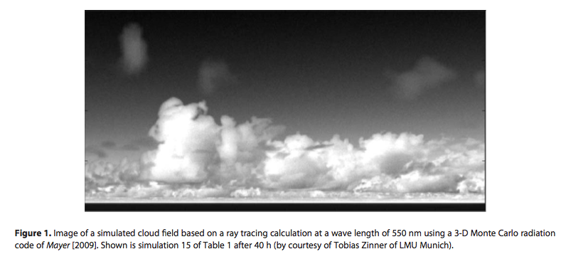
From Seifert et al 2015
Figure 2 – Click to expand
It is an involved paper, but here is one of the conclusions, relevant for the topic at hand:
Our simulations suggest that parameterizations of cloud-aerosol effects in large-scale models are almost certain to overstate the impact of aerosols on cloud albedo and rain rate. The process understanding on which the parameterizations are based is applicable to isolated clouds in constant environments, but necessarily neglects interactions between clouds, precipitation, and circulations that, as we have shown, tend to buffer much of the impact of aerosol change.
For people new to parameterizations, a couple of articles that might be useful:
Conclusion
Climate models necessarily have some massive oversimplifications, as we can see from the large eddy simulation which has 25m x 25m grid cells while GCMs have 100km x 100km at best. Even LES models have simplifications – to get to direct numerical solution (DNS) of the equations for turbulent flow we would need a scale closer to a few millimeters rather than meters.
The over-simplifications in GCMs require “parameters” which are not actually intrinsic material properties, but are more an average of some part of a climate process over a large scale. (Note that even if we had the resolution for the actual fundamental physics we wouldn’t necessary know the material parameters necessary, especially in the case of aerosols which are heterogeneous in time and space).
As the climate changes will these “parameters” remain constant, or change as the climate changes?
References
Cloud tuning in a coupled climate model: Impact on 20th century warming, Jean-Christophe Golaz, Larry W. Horowitz, and Hiram Levy II, GRL (2013) – free paper
Twentieth century climate model response and climate sensitivity, Jeffrey T. Kiehl, GRL (2007) – free paper
Large-eddy simulation of the transient and near-equilibrium behavior of precipitating shallow convection, Axel Seifert et al, Journal of Advances in Modeling Earth Systems (2015) – free paper


Excellent Post, especially for someone such as I who never thought about all these complexities introduced by clouds. Any feelings about how much uncertainty this introduces into future average Earth temperature projections? Experimental results are perhaps the best to go on.
I was impressed by those Berkeley Earth results for temperature measurements going back into the 1800’s…..What does Science of Doom and others think of graphs such as the one accessed at: ?
https://images.search.yahoo.com/search/images?p=berkely+earth+graphs&fr=mcafee&imgurl=https%3A%2F%2Fwattsupwiththat.files.wordpress.com%2F2012%2F07%2Fberkeley-earth-temperature-and-volcanoes.jpg%3Fw%3D720#id=0&iurl=https%3A%2F%2Fwattsupwiththat.files.wordpress.com%2F2012%2F07%2Fberkeley-earth-temperature-and-volcanoes.jpg%3Fw%3D720&action=click
Curious: Before 1850, the standard method of putting a thermometer in a isolated shaded passively-ventilated enclosure was not used. This became standard practice in most locations between 1850 and 1900. When BEST goes back before 1850, they are entering a period without standard measurement practices and large correction factors. I wonder whether there methodology can properly align data with such serious problems. Whatever you believe, take their expanding confidence interval very seriously.
curiousdp,
I haven’t looked into the accuracy or uncertainty of the global temperature reconstructions. Because I know that different people with different approaches (including Berkeley who came to it as an outsider group) have looked at the data and appear to have almost identical reconstructions I assume that they are probably roughly correct.
On your first question:
Compared with? A model is a simplification. It wasn’t a revelation to me finding more details on this particular aspect of the simplification.
The question might be rephrased:
What uncertainty into future average Earth temperature projections do sub-grid parameterizations introduce?
My answer so far: “Quite a bit”. Perhaps too many significant figures in that answer, I don’t want to give an idea of super-accuracy..
Climate scientists are doing experiments all the time. One part of the blogosphere imagines that 99% of climate scientists sit around supercomputers, get the output and make pronouncements. (I’m not saying you think this, I just can’t resist the opportunity to mock the idea).
The earth is a big place and measuring microphysics processes across all settings is extremely challenging. There have been lots of satellites in the last 15 years to give detailed measurements of a large number of variables (including aerosol parameters) across most of the globe often on a daily basis. This helps to uncover a lot of relationships. Then there are lots of field experiments to dig into various parameters. And then there are approaches of using higher resolution models on shorter time periods across a smaller region to get a better understanding of various relationships and to find and correct flaws in GCMs’ parameterizations.
There is one massive experiment running at the moment, but we won’t get the results for some time.
Well, we’re getting one result in about a week… February 2017 is going to have a really high anomaly. Exactly what one would expect on the way to a really warm year… maybe even the 4th warmest in a row. And, SSH as of Nov 30, 2016… a La Niña period… was at its highest level in the satellite record. OHC has backed off a bit, but it’s on its way back up.
SOD: If you are getting back into models, this might make an interesting post.
Ming Zhao, J.-C. Golaz, I. M. Held, V. Ramaswamy, S.-J. Lin, Y. Ming, P. Ginoux, B. Wyman, L. J. Donner, D. Paynter, and H. Guo, 2016: Uncertainty in Model Climate Sensitivity Traced to Representations of Cumulus Precipitation Microphysics. J. Climate, 29, 543–560.
doi: http://dx.doi.org/10.1175/JCLI-D-15-0191.1
Uncertainty in equilibrium climate sensitivity impedes accurate climate projections. While the intermodel spread is known to arise primarily from differences in cloud feedback, the exact processes responsible for the spread remain unclear. To help identify some key sources of uncertainty, the authors use a developmental version of the next-generation Geophysical Fluid Dynamics Laboratory global climate model (GCM) to construct a tightly controlled set of GCMs where only the formulation of convective precipitation is changed. The different models provide simulation of present-day climatology of comparable quality compared to the model ensemble from phase 5 of CMIP (CMIP5). The authors demonstrate that model estimates of climate sensitivity can be strongly affected by the manner through which cumulus cloud condensate is converted into precipitation in a model’s convection parameterization, processes that are only crudely accounted for in GCMs. In particular, two commonly used methods for converting cumulus condensate into precipitation can lead to drastically different climate sensitivity, as estimated here with an atmosphere–land model by increasing sea surface temperatures uniformly and examining the response in the top-of-atmosphere energy balance. The effect can be quantified through a bulk convective detrainment efficiency, which measures the ability of cumulus convection to generate condensate per unit precipitation. The model differences, dominated by shortwave feedbacks, come from broad regimes ranging from large-scale ascent to subsidence regions. Given current uncertainties in representing convective precipitation microphysics and the current inability to find a clear observational constraint that favors one version of the authors’ model over the others, the implications of this ability to engineer climate sensitivity need to be considered when estimating the uncertainty in climate projections.
The paper is behind a paywall, but the poster presentation is not
Click to access Zhao_CFMIP_2015.pdf
According to the poster, “drastically different climate sensitivity” includes climate feedback parameters of 0.48-0.82 K/W/m2 (ECS 1.7-3.0 K/doubling.)
Frank,
A very interesting paper, worth another article along with some other papers they cite in the family.
From their conclusion:
Ever increasing model resolution along with process studies may finally bring these questions to a conclusion. Somewhere between the end of this decade and the time when supercomputing power has increased by a factor of a trillion or so.
You know when you are there (actually a little after: because the results stop changing; the process studies back up the formulas; and the empirical results match the model simulations), but not before.
Sometime I will try and write an article to illuminate the issue to people who can’t picture how models, model resolution and parameterizations create a fog of confusion..
Just a few of the interesting papers cited in the above paper as part of the family of trying to zero in on reality:
Missing iris efect as a possible cause of muted hydrological change and high climate sensitivity in models, Thorsten Mauritsen and Bjorn Stevens, Nature Geoscience (2015) – free paper
Clouds, circulation and climate sensitivity, Nature, Bony et al (2015) – free paper
Spread in model climate sensitivity traced to atmospheric convective mixing, Nature, Sherwood et al, (2014) – free paper
What Are Climate Models Missing?, Stevens & Bony, Science (2013) – free paper
Obviously Nature and Science think these papers are high quality (they are very discriminating journals).
I’m a layperson, but I’ve read all of those. If I find a paper interesting, I follow the cites. So every week I check to see who has cited my list. Recently I found this 2017 paper, pay walled, that cites the Stevens Iris paper:
… Applying this approach to tropical remote sensing measurements over years 2000–2016 shows that an inferred negative short-term cloud feedback from deep convection was nearly offset by a positive cloud feedback from stable regimes. …
SOD: Thanks for the linked papers. The differences between models of a simple aqua planet in Stevens and Bony shows just how “wrong” most models must be – because at most one of these four is right.
When feeling sarcastic, I’d say that the greatest climate change catastrophe since the last ice age was the desertification of the Sahara. I’d believe predictions of future catastrophe only when GCMs were able to explain this part of the past. The Bony Nature paper takes this problem seriously.
I’ve become obsessed (often a bad idea) with the idea that simple physics links climate sensitivity to a slow down in convective turnover of the atmosphere. An ECS of 3.7 K/doubling implies an increase in net TOA flux of only 1 W/m2/K. At constant relative humidity, latent heat transport at the surface (80 W/m2) increases at 7%/K or 5.6 W/m2K. IF that 5.6 W/m2/K increase in latent heat continues to be transported to the upper troposphere (where it can escape to space as LWR), then incoming SWR must increase by 4.6 W/m2/K. Since current albedo reflects about 100 W/m2 of incoming SWR, this would require an unrealistic 4.6%/K decrease in reflected SWR. Net radiative cooling of surface (OLR-DLR) does not change appreciably with surface temperature. So, for climate sensitivity to be high, this 7%/K increase in absolute humidity near the surface can not be carried upward at the current rate of atmospheric turnover.
This provides an alternative to the standard way of approaching climate sensitivity, summing Planck, water vapor, lapse rate, cloud and surface albedo feedbacks (in terms of W/m2/K).
Frank,
Assuming ECS means equilibrium climate sensitivity, net TOA flux at equilibrium would be zero, not one W/m². If you mean the instantaneous flux change for a step doubling of CO2, the net TOA flux would decrease, not increase.
It doesn’t. The scale height of water vapor is 2km. 99.3% of all water vapor in the atmosphere is below 10km. Most latent heat is transferred to the atmosphere in the first 4km. Except in large storms, there is little latent heat transfer above the middle of the troposphere.
Frank,
Increasing precipitation with temperature means that the surface temperature doesn’t go up as fast, i.e. lower ECS, because you have latent heat transfer replacing radiative heat transfer to keep the energy balance. Precipitation is not an independent variable.
Frank,
To put it another way: If you have an ECS of 3.7K/doubling, then you can’t have precipitation increasing at 7%/K. That sort of increase would mean an ECS well below 2K/doubling.
The 4 papers provide some interesting contrasts, probably worth an article.
One of the papers, Sherwood, Bony & Dufresne (2014) say:
Which is quite a different perspective from Mauritzen.
Then, Uncertainty in Model Climate Sensitivity Traced to Representations of Cumulus Precipitation Microphysics, Ming Zhao et al, Journal of Climate (2016):
SOD, I would interject a note of caution concerning increasing spatial resolution in turbulent simulations. The cultural prejudice among modelers is that if we could only run a fine enough grid and had a big enough computer we would resolve “all scales” and get the “right” answer. There is some recent evidence of a disturbing lack of grid convergence in LES simulations of turbulent flows. There is still a lot of very hard work to do before we get a handle on these issues.
Also bear in mind that convection is a classical ill posed problem due to the turbulent shear layers. It’s of course an interesting area for people to work on, but also quite challenging.
I thought I would point out that Nic Lewis has a summary writeup on ECS that includes in its later parts what I found some interesting points on convection in GCM’s and also on clouds.
Click to access briefing-note-on-climate-sensitivity-etc_nic-lewis_mar2016.pdf
dpy6629,
Sorry for my slow reply, I have been travelling.
I had a read of Nic Lewis’ article, very interesting.
You also say:
There is a big difference between Large Eddy Simulation (LES) – which still contains some important parameterizations for closure of the equations – and Direct Numerical Simulation (DNS).
So do modelers believe getting to LES would get the right answer, or we need to get to DNS?
If we could do DNS then the answers would still depend on initial conditions and selection of material properties and perhaps we would be no further along due to having to run 1 trillion ensembles of initial conditions.. (I don’t know the answer).
And perhaps we would still have convergence issues?
Any comments?
SOD, I thought I made a comment last night but it seems to have disappeared for some reason. In any case, the problem here is that LES and DNS are an area of deep ignorance. The simulations are too expensive to do real validation studies. In any case, theoretical understanding is lacking. High quality data is lacking too.
The real issue for all these eddy resolving simulations is the nature of the attractor. Next to nothing is known. Rigorous bounds on attractor dimension are huge — O(Reynolds#). How attractive is the attractor? Critical question for numerical simulations. We know nothing really. What does “convergence”mean in a time dependent context? We know next to nothing.
We do know there will be bifurcations and saddle points where the “climate” of the system will be very sensitive to initial conditions. In terms of evaluating discrete simulations, one really serious problem here is that standard error control methods fail for time accurate chaotic simulations because the adjoint diverges. Just chopping the time step and seeing that the changes are not too large is not adequate.
So in a state of ignorance, people tend to fall back on cultural prejudice or scientific arrogance or colorful fluid dynamics. It’s very dangerous. The problem here is that the computational resources demanded by this faith based approach are huge. In the absence of better understanding, that may be a huge waste of resources. Just throwing darts at a picture of James Hansen with a halo, who was one of the originators of the dubious idea that if I run a weather model for centuries on a very course grid, the answers mean something.
For climate simulations, these methods will be impossible for your and my lifetime and possibly forever depending on the nature of the attractor. You are digging into some of the technical details of subgrid parameterizations of ill posed processes such as convection and precipitation.
I personally think there is an opportunity to use simpler models to help us understand the nature of the problem and establish parameters for further research. And we need to improve our theoretical understanding of the Navier-Stokes equations. There are promising theoretical ideas here. Instead, we are wasting billions on research projects that just “run the models” and then draw dubious conclusions. The climate science establishment is all in on this self-serving research plan.
An excellent example of how colorful fluid dynamics can be used to serve political interests is Gavin Schmidt’s most recent post at Real Climate. AOGCM’s are used along with fingerprinting to “prove” that recent warming is almost all due to CO2 increases. But, AOGCM’s get the detailed patterns wrong, including SST warming patterns, TMT, topical TMT, and indeed GMAT too if you focus on the last few years. How the fingerprints are supposed to be meaningful is beyond my comprehension. Schmidt insists that AOGCM’s are not tuned to GMAT even though it seems to be rather good for the historical period in CMIP5 runs. I don’t believe that modelers just ignore this historical record.
In any case, its hard to ignore Nic Lewis’ statement that
You can see in Nic’s writeup on ECS what some of the serious problems are. Basically, by changing parameters controlling precipitation and clouds, you can get a wide range of ECS and SST patterns. No one has offered a convincing argument as to why AOGCM’s offer meaningful scientific evidence of much.
dpy6629,
+ many
Even worse, most of the models are minor variations of the same basic model. I believe the word ‘mathturbation’ applies.
The question of evaporation & precipitation in a warming climate is also worth a separate article. At the moment I don’t understand it. That is, there is a constraint or two that I am not understanding when I read papers talking about it.
SOD,
Thanks for a thoughtful exposition, as well as the links. I am encouraged that there is at least some acknowledgement in the papers of 1) a lack of progress by the models in reducing uncertainty in climate sensitivity, 2) that empirical estimates of sensitivity generally fall well below the model average, and 3) that it is crucially important for developing sensible public policy to accurately quantify the value for climate sensitivity.
My personal guess is that empirical estimates will lead the way in narrowing the plausible range for sensitivity (just as they have so far), especially if uncertainty in aerosol effects (direct and indirect) can be modestly narrowed. Models, if substantially improved, are more likely to contribute to estimating how precipitation will change, both globally and regionally.
SOD, Thank you for writing this very good post. I have two comments.
1. You quote Golaz et al 2013 “Cloud tuning in a coupled climate model: Impact on 20th century warming”, as citing Andrews et al 2012 as well as Kiehl et al 2007 and Schwarz et al 2007 as showing that global climate models exhibited inverse correlation between forcing and sensitivity. The relevant forcing by far here is aerosol forcing. The absolute level of forcing from CO2 matters little since the ratio of CO2 concentration to preindustrial will be the same for all models for equilibrium climate sensitivity (being 2x) and for their historical simulations. While Kiehl showed a significant negative correlation between aerosol forcing and sensitivity in CMIP3 models, little such correlation exists in CMIP5 models.
Andrews et al 2012 did not in fact look into the ECS – aerosol forcing correlation, but Forster et al 2013 JGR did, and found it far weaker than in CMIP3 models. The explanation of the weak (negative) correlation between aerosol forcing and ECS in CMIP5 models is that they exhibit a very large spread in warming over the historical period. Models with low aerosol forcing (primarily, those with no indirect aerosol effect) generally warm faster than observed. The main exceptions are the inmcm4 model, which has the lowest ECS of all CMIP5 models (about 1.9 K), and the two GFDL-ESM2 models, which have very low TCR to ECS ratios.
2. Thank you for drawing attention to the Siefert et al paper. Its finding that aerosol indirect forcing is probably minor, and much weaker than simulated by GCMs that include it, is consistent with the beliefs of Graeme Stephens, who has very extensive knowledge of clouds, particularly from the observational side. He has said that he would recommend incorporating no indirect aerosol forcing in it. That is what Siefert’s co-author Bjorn Stevens, another great cloud expert, did in the MPI CMIP5 models.
A consequence of indirect aerosol forcing being zero would be that to match historical warming a GCM would need to have a very low TCR – of the order of 1.2 K, if other AR5 forcing data are realistic.
Nic wrote: “Andrews et al 2012 did not in fact look into the ECS – aerosol forcing correlation, but Forster et al 2013 JGR did, and found it far weaker than in CMIP3 models. The explanation of the weak (negative) correlation between aerosol forcing and ECS in CMIP5 models is that they exhibit a very large spread in warming over the historical period.”
This information is inconsistent with Figure 10.5 of AR5 WG1, which shows that high warming from GHGs must be offset by high cooling from aerosols. There is no other way to get much tight error bars for total anthropogenic warming than for either of its components. In Table 3 of Forster (2013), I find that there is a fair correlation (R2 0.32) between Hist GHG 2003 (warming caused by GHGs) and Hist NonGHG 2003 (net cooling caused by nonGHGs = aerosols, land use, O3). This agrees with what one would expect from Figure 10.5.
Nevertheless, Forster’s Figure 9 shows no correlation between the amount of warming produced by a model and its climate feedback parameter (alpha), its ocean heat uptake efficiency (kappa) or the sum of these two, climate resistance (rho). How can this be? I think these values have been obtained from 4XCO2 experiments. If I understand correctly, many models do not behave as if these parameters are constant with time or the same in TCR and 4XCO2 runs. Historical warming is most closely related to the 1% pa model runs used to calculate TCR. I’d guess that if one knew alpha, kappa and rho for TCR runs, we’d probably see a relationship between aerosol cooling and rho.
If I look at the adjusted forcing (ie W/m2, instead of K) through 2003 from GHGs and from nonGHGs, there is almost no correlation. So the correlation appears only with warming (forcing times TCR). With all of the different kinds of forcing and imperfections with mathematic models of GCM output, I don’t really understand this stuff very well. Nor can I explain why there is so much scatter in 2003 warming in the GRL paper 1.0 K (0.4-1.5 K, 90% ci) and less scatter in Figure 10.5, 0.7 K (0.6-0.8 K, 70% ci). The difference in warming is because Figure 10.5 covers 1951-2000, while the GRL paper covers the historical period (1860-2003). Then we have the added complication that the GRL paper doesn’t clearly separate aerosol cooling from other nonGHG factors (land use and ozone) and Figure 10.5 doesn’t tell us where land use and ozone enter the picture.
The GFDL CM3 model showed only 0.3 K of warming since 1860 in the GRL paper. I wonder how much warming it showed from 1951-2000? Could it have been discarded as an outlier?
Intuitively, it seems possible tune a model with too high an ECS (too little additional heat escaping to space per K increase in Ts) by sending the extra heat into the ocean – if you haven’t handled the problem with aerosols. So there are at least two opportunities for tuning overall warming given a fixed ECS. (I think we’ve discussed this before). In Figure 10.5, the models appear to have been tuned to attribute 100% of 1951-2000 warming to man. Consequently 1860-2003 runs can have widely scattered warming, without interfering with the all-important human attribution statement. (This statement may reflect paranoid fantasy brought on by reading too many skeptical blogs.)
Figure 10.5 | Assessed likely ranges (whiskers) and their mid-points (bars) for attributable warming trends over the 1951–2010 period due to well-mixed greenhouse gases, other anthropogenic forcings (OA), natural forcings (NAT), combined anthropogenic forcings (ANT) and internal variability.
Frank
A quick response as I am about to go out.
You say re AR5 Fig 10.5 “There is no other way to get much tight error bars for total anthropogenic warming than for either of its components.”
I don’t think that’s right. Fig. 10.5 is based on spatiotemporal pattern regression. It is much easier to separate responses to natural forcings (which are cyclical or episodic) from those to anthropogenic forcings than to separate responses to GHG forcing from responses to non-GHG anthropogenic forcings, all of which have magnitude time series that are nearly colinear with those for GHG forcing.
Frank [wrongly] wrote about AR5 Fig 10.5 “There is no other way to get much tight error bars for total anthropogenic warming than for either of its components.”
Nic replied: I don’t think that’s right. Fig. 10.5 is based on spatiotemporal pattern regression.
Thanks Nic. I see that Figure 10.5 (which is derived from 10.4) uses “fingerprinting” from model output to attribute OBSERVED warming into GHG and non-GHG components and the error bars may reflect the uncertainty inherent in this attribution. I thought this Figure summarized how models hindcast similar amounts of total warming from very different amounts of GHG warming and aerosol cooling.
For best I can tell, attribution of observed warming using fingerprinting simply reflects the biases of the models used Figure 10.4 and merely rescales their output to match observed output. CMIP performed three hindcasts of 20th century warming those results are found in Table 3 of Forster (2013). The multi-model means (90% cl) are:
1.0 +/- 0.6 K [1860-]2003 Hist (with all forcings)
1.4 +/- 0.4 K [1860-]2003 HistGHG (with only WMGHG)
0.1 +/- 0.2 K [1860-]2003 HistNat (with only solar and volcanic)
-0.5 +/- 0.6 K [1860-]2003 HistNonGHG (difference)
So this output conveys almost the same message as Figure 10.5 except – as you pointed out – the error bar for all modeled warming – is far wider than for ANT. So there is far less evidence supporting tuning than I thought, though – as I noted above – there is still a modest negative correlation between HistGHG and HistNonGHG.
I looked up IPCC’s 1951-2010 range in Jones (2013) to see if it was different from 1860-2003:
0.65 K 1951-2010 HADCRUT4
0.74 (0.38-1.12) K 1951-2010 Hist (with all forcings)
1.12 (0.88-1.64) K 1951-2010 HistGHG (with only WMGHG)
-0.08 (-0.35-+0.09) K 1951-2010 HistNat (with only solar and volcanic)
-0.30 K 1951-2010 HistNonGHG (difference)
Models HINDCAST 1.12 (0.88-1.64) K warming due to WMGHGs only but ATTRIBUTE only 0.9 (0.5-1.3) K of observed warming to WMGHGs through fingerprinting. (:)) No wonder I am confused.
Nic,
Interesting comments.
I’m travelling and left my notes behind.. I did start to look at the direct aerosol forcing from a number of estimates and there was quite a range. It led me to think that even with zero indirect aerosol forcing, climate sensitivity would still be quite varied across models. However, I hadn’t got too far with a review.
How did you reach this conclusion?
SoD,
To clarify, this comment of mine was based on assuming that forcings in the GCM matched best estimates per AR5, save for indirect aerosol forcing being zero. Obviously, if a GCM had very strong direct aerosol forcing, or unrealsitically low GHG forcing, it would be able to match historical warming with a higher TCR.
Fig. 7.19(b) of IPCC AR5 WG1 shows the uncertainty in direct aerosol forcing (RFari) estiamted for CMIP5 models. The median is ~ -0.45 W/m2; the 17th percentile is ~ -0.6 W/m2.
SOD and Nic: When I was wading through the material related to Figure 10.5 above, I ran across Figure S5 from Jones (2012)
http://onlinelibrary.wiley.com/store/10.1002/jgrd.50239/asset/supinfo/2012JD018512text01.pdf?v=1&s=4c06b6723d2a80b7133a543597716d3c2da59d6c
“Figure S5. (a) Global annual mean TAS anomalies, relative to 1880-1919, for CMIP3 and CMIP5 historical simulations, split into those simulations that include and not include indirect aerosol influences.”
Models without indirect aerosol effect warmed 0.2 K (0.05 K/decade) more than models with indirect aerosol effect. This gap developed between 1940 and 1980: 0.34 K vs 0.14 K of warming in the multi-model mean in this period.
“Figure S5. b) Spatial trend maps of weighted means of models for the 1901-2010 (Left) and 1940-1979 (Right) periods. First row shows the average trend of the models including direct sulphate aerosol effects and the second row the average trend of the models with direct and indirect aerosol effects.”
Models without indirect aerosol effect show warming 0-0.05 K/decade of warming during 1940-1979 almost everywhere except polar regions. Models with aerosol indirect effect show cooling of 0 to -.05 K/decade on all continents and most NH temperate oceans, with some regions cooling -0.05 to -0.10 K/decade.
Nick Stoke’s trend viewer for the same period:
global – land – ocean (K change 1940-1980)
HadCRUT -0.08; CRUTEMP4 -0.07; HADSST3 -0.10
GISSlo -0.02 GISSTs +0.11
NOAAlo -0.02; NOAAla +0.02; NOAAsst -0.05
BESTlo -0.06; BESTla -0.05;
Unfortunately this period begins with the suspect SSTs during WWII and includes most of the full amplitude of the fall in AMO (0.25? K), which climate models presumably don’t replicate. So, with the indirect aerosol effect and cancelled AMO, models might predict a fall of -0.1 K and without a rise of +0.1 K – along with large land/ocean and NH/SH differences. (And these hindcasts might be biased high if the average model has a climate sensitivity that is too high).
The observations don’t conclusively favor either type of model. The spatial pattern of temperature change over this period might be more informative, but the authors (suspiciously?) didn’t provide a spatial pattern for observed warming during 1940-1979.
The complications from the AMO might be eliminated by studying 65-year periods from trough to trough (1915-1980?) and/or peak to peak (1940-2005?) that include the period of biggest change in indirect aerosol forcing (1940-1980).
SOD said: “If we could do DNS then the answers would still depend on initial conditions and selection of material properties and perhaps we would be no further along due to having to run 1 trillion ensembles of initial conditions.. (I don’t know the answer).”
In case you have forgotten, Isaac Held had an interesting post and video on resolving ocean eddies that covered some basic principles about scale.
https://www.gfdl.noaa.gov/blog_held/29-eddy-resolving-ocean-models/
As for initialization, my guess is that we don’t need an ensemble with a trillion runs. The rational? Imagine picking different starting years in the instrumental record as a model for picking different initialization conditions. When energy balance models are used to calculate TCR over the past 130 or 65 years (Lewis and Curry 2014) or the past for 40 year and decades in the past 40 years (Otto 2013), we obtain roughly the same answer. IMO, the Pause in the first decade of the 2000s has lost its significance: the trend in the two decades before and after 1998 are essentially the same. So, if picking different starting years in history is a good model for different initializations of an AOGCM, I think we are likely to reach about the same average future in about 50 years (but not a decade or two).
For a long-term perspective (more than a century), the instrumental period is too short. The combined ice core record from both poles during the Holocene (for a longer perspective) might be useful. Unfortunately, we don’t know how much of the variability in that record is naturally-forced, and how much is unforced variability (like ENSO and other phenomena we see in the instrumental record such as the AMO) and how much is forced.
However, if we are on the verge of some chaotic bifurcation or tipping point my rationalization is meaningless. Descent into another ice age? Massive release of methane? We have experience catastrophic climate change during the Holocene – desertification of the Sahara.
There has been some attention to a paper from Tan et. al 2016. Observational constraints on mixed-phase clouds imply higher climate sensitivity
Ivy Tan, Trude Storelvmo, Mark D. Zelinka. They claim that climate models are bad at calculating ice particles and water droplets, and that they get the radiation budget wrong. Ivy Tan: “The supercooled liquid fraction (SLF) of these clouds is severely underestimated by a multitude of global climate models (GCMs) relative to measurements obtained by satellite observations.” and “The higher ECS estimates are linked to a weaker “cloud phase feedback.” This negative feedback mechanism operates by decreasing the cloud glaciation rate, resulting in optically thicker and more reflective supercooled liquid clouds as the troposphere deepens in response to warming, at a rate that depends on the SLF prior to carbon dioxide doubling. The feedback is shown to be too strong in climate models that underestimate SLF relative to observations, thereby leading to underestimates of ECS.”
I think the questions are important. How do supercooled water droplets and ice particles increase or decrease in the atmosphere as the climate change, and what impact will it have on radiation. Will the atmosphere be optically thinner than models assume, and what do models assume?
From Yale University: http://climate.yale.edu/penumbra/topic/59 “The work by Storelvmo’s group suggests that scientists may actually be close to designating the lower values in the currently accepted range as being “unlikely.” According to Michael Mann, Distinguished Professor of Atmospheric Science at Penn State University, the latest studies “provide sobering evidence that Earth’s climate sensitivity may lie in the upper end of the current uncertainty range.”
The research published today in Science by Storelvmo, her graduate student Ivy Tan, and Mark Zelinka of Lawrence Livermore National Laboratory (Tan et al, 2016) analyzes satellite measurements to conclude that the middle and upper troposphere contain a higher ratio of water to ice than was previously believed. The water is present in the form of super-cooled droplets; the ice, in tiny crystals. The ratio of water to ice is critical because tiny water droplets are highly reflective of incoming sunlight and ice crystals are not. A higher liquid fraction in the upper atmosphere means greater reflection of incoming solar radiation: less sunlight and heat reach the Earth’s surface and there is less warming. This is a classic example of negative feedback in the climate system: as the atmosphere starts to warm because of increased greenhouse gases, a mechanism sets in to dampen the effect—in this case, suspended ice crystals in the upper troposphere melt into tiny water droplets that reflect solar energy back into space.
Current climate models correctly simulate this effect by replacing ice with water as the world warms, but these models appear to have overestimated the actual availability of ice. Less ice to melt means that less water will form to brighten the atmosphere. The latest findings by Storelvmo and her colleagues indicate that much of the incoming solar radiation that today’s models predict will be reflected back to space (as tropospheric ice converts to water) will actually pass through the atmosphere and heat the Earth.
To calculate how much additional heating will occur, the authors configured the National Center for Atmospheric Research’s Community Atmosphere Model (CAM 5.1) to calculate equilibrium climate sensitivity using a range of atmospheric water-to-ice ratios based on the latest satellite estimations. The newly constrained model predicted an equilibrium climate sensitivity (ECS) of between 5.0 and 5.3 degrees, compared to an estimate of 4.0 degrees using the conventional water-to-ice ratio. Storelvmo expects that when other researchers adjust their respective models to reflect appropriate proportions of ice and water in mixed-phase clouds, all of their ECS values will shift upward.
The implications of higher ECS are profound, and might already be making themselves felt were it not for a different phenomenon described by Storelvmo earlier this month in a paper in Nature Geoscience (Storelvmo et al 2016). That study used ground-based measurements of incoming solar radiation to determine that highly reflective sulfate aerosols in the atmosphere—which have both natural (volcanic activity) and man-made (burning of high-sulfur fuels) origins—can mask the full warming effect of carbon dioxide. Using mathematical techniques from econometrics, Storelvmo and her colleagues, Thomas Leirvik of the University of Norland (Norway), Ulrike Lohmann and Martin Wild of ETH Zürich, and Peter Phillips of Yale, attempted to disentangle the competing influences of carbon dioxide and sulfates in the record of recent temperature changes. Their analysis determined that existing levels of sulfate aerosols have counteracted about 0.5 degrees Centigrade worth of warming that would otherwise have occurred in the last few decades.”
I suspect this to have a big acticvist fingerprint, as it cannot show the changes in ice crystals and water droplets over time. They cannot show satellite measurements, even when that should be the data they use. And there is some confusion in the presentations of the study. Some say thar ice particles don`t matter, and it is when the atmosphere heats and they turn into droplets that it has cosequences on incoming radiation. some say that the more ice you have in the upper atmosphere, the less warming there will be on the Earth’s surface.
Something for SoD and other readers to get a sober glance at?
Take Home Messages from the study: https://calipsocloudsat.sciencesconf.org/conference/calipsocloudsat/pages/Trude_STORELVMO.pdf
And nothing about the real and historical change of supercooled liquids and particles in the atmosphere.
I have tried to see if there is any observations of cloud change over time. Found this: Evidence for climate change in the satellite cloud record
Joel R. Norris, Robert J. Allen, Amato T. Evan, Mark D. Zelinka, Christopher W. O’Dell & Stephen A. Klein.
“Observed and simulated cloud change patterns are consistent with poleward retreat of mid-latitude storm tracks, expansion of subtropical dry zones, and increasing height of the highest cloud tops at all latitudes. The primary drivers of these cloud changes appear to be increasing greenhouse gas concentrations and a recovery from volcanic radiative cooling. These results indicate that the cloud changes most consistently predicted by global climate models are currently occurring in nature.”
This should show another story than Tan et al. And Mark D. Zelinka on both of them. Speaking with two tongues?
NK: I’d again recommend that you look the paper linked below, which shows how poorly AOGCMs reproduce the large feedbacks associated with the 3.5 K seasonal increase in GMST. IMO, the first step to understanding the significance the output of models – and especially one or a few models is to see how poorly they reproduce large seasonal changes. Then remember than the models behave the way they do because parameters have been tuned. SOD has a nice article on model tuning at the other link below:
http://www.pnas.org/content/110/19/7568.full
Furthermore, when discussing model tuning at RealClimate, Gavin has said that refining a reasonably-tuned model to improve the performance in some area (say high cirrus cloud) often leads to poorer performance in other areas. Parameters interact with each other in surprising ways, so tuning parameters one-by-one doesn’t lead to a global optimum. A model with more realistic cirrus clouds is not necessarily a better model for predicting temperature and precipitation at various locations on the planet. (Perhaps I’m overly skeptical, but scientists are supposed to be skeptical.)
NK: Climate models are tuned to reproduce today’s climate. If the parameterization of clouds in an AOCGM needs to be modified so they contain less ice (and therefore have a smaller albedo), then other model parameters will need to be adjusted so that a final revised model will exhibit today’s albedo. Speculating about the output of a final revised model that properly represents ice in clouds AND today’s climate seems pretty worthless to me – but it will get you published in Science and praised by those convinced catastrophe is coming. (The same thing wouldn’t happen if these changes had lowered climate sensitivity.) Perhaps CMIP 6 models with modified clouds will exhibit ECSs of around 5.0! In that case, the difference between models and observations will be far greater than it is today and we will have conclusively proved that models are invalid!
The same arguments apply to the slight change in albedo due to a poleward shift in storm tracks on warming.
Cynicism and sarcasm aside, I suggest you look at the PNAS paper below, which compares cloud feedbacks during the annual seasonal temperature cycle. (One of the authors, Manabe, pioneered the GFDL climate model.) Due to the difference in heat capacity between the hemispheres, the average location in the NH warms about 10 K during its summer while the SH is cooling only 3 K. The resulting 3.5 K change in GMST is associated with large, feedbacks that have been observed many times in the satellite era. This paper shows how well current climate models are able to reproduce these feedbacks, especially cloud feedback. No models do a particularly good job reproducing today’s seasonal feedbacks AND they disagree significantly with each other. When we have some models that do a good job of reproducing what we observe from space (during the seasonal cycle and at other times), then I will worry more than I currently do about the possibility ECS is well above 2 K. Others may choose to respond to all of the ups and downs on what is likely to be a long scientific journey.
http://www.pnas.org/content/110/19/7568.full
Frank: Thank you for your replies.
I folow you in this: ” If the parameterization of clouds in an AOCGM needs to be modified so they contain less ice (and therefore have a smaller albedo), then other model parameters will need to be adjusted so that a final revised model will exhibit today’s albedo. Speculating about the output of a final revised model that properly represents ice in clouds AND today’s climate seems pretty worthless to me – but it will get you published in Science and praised by those convinced catastrophe is coming.”
My point is that there is still so much uncertainty in basic parameterization of clouds (and ocean) that all models will necessarily be wrong. Each model will have a lot of parameters combined. So I cannot imagine how one can trust it when it comes to “projections” into a distant future. Or to trust an ensemble, with many of the biased parameters in common.
I am also sceptic to the Tsushimaa and Manabeb article when they say: “Here, we show that the gain factors obtained from satellite observations of cloud radiative forcing are effective for identifying systematic biases of the feedback processes that control the sensitivity of simulated climate, providing useful information for validating and improving a climate model.”
I suspect them to be far to optimistic in this, when I look at the difficulties to measure scattering, absorption and emission from all the types of clouds, how clouds change over short periods, and to calculate feedbacks..
And thank you for the reference Frank. I think it shows how climate models are systematically biased when it comes to cloud radiative forcing, But I don`t know if it will help very much to get it right.
Some precision of my latest comment. I think the working with gain factors can give some better hindcast, and some better predictions for the first decades. But to fix some weaknesses doesn`t mean that it will be right (as to have a long predictive value). As for weather forecasts which have no value for more than ca 10 days.
NK wrote: I am also sceptic to the Tsushima and Manabe article when they say: “Here, we show that the gain factors obtained from satellite observations of cloud radiative forcing are effective for identifying systematic biases of the feedback processes that control the sensitivity of simulated climate, providing useful information for validating and improving a climate model.”
I suspect them to be far to optimistic in this, when I look at the difficulties to measure scattering, absorption and emission from all the types of clouds, how clouds change over short periods, and to calculate feedbacks.
I find it very encouraging to read that an influential modeler like Manabe thinks AOGCMs need “validating” and “improving” and has focused on the large and reproducible signals associated with the seasonal cycle when trying to do so. I find that much more enlightened that those who focus on one aspect of model and make predictions about what will happen when that aspect is improved.
As for being “overly-optimistic”, I think that every scientist needs to be an optimist (and have a fairly sizable ego) to think that he can make a contribution that will solve an important problem (which earlier workers have often failed to solve). With luck, however, even failure to reach the ultimate goal will move us forward a little in some area. Unfortunately, policymakers need unambiguous answers and scientists can’t deliver them on a schedule.
nobodysknowledge,
Thanks for this comment, it is informative.
It seems that Tan et al. have made a valuable contribution to basic science. Unfortunately, they have to contaminate it with meaningless speculation as to the effect on climate sensitivity. The Yale quote: “The work by Storelvmo’s group suggests that scientists may actually be close to designating the lower values in the currently accepted range as being unlikely” is just politics. The lower part of the IPCC range is based on observational data, not models, so there is no reason the new results should have any effect on that part of the range. No doubt the new results will cause some upward shift in model sensitivity. When it comes to feedbacks, the modellers know how to add but not how to subtract. So they will likely include this while continuing to ignore negative feedbacks like Lindzen’s Iris Effect.
Mike M. The observations that I cited above should point to some negative feedbacks: What did CAM 5.1 model get out of these?
“poleward retreat of mid-latitude storm tracks” should give higher consentrations of water wapor, ice particles and water droplets in higher altitudes toward the poles.
“expansion of subtropical dry zones” should give some more subtropical IR radiation at TOA.
“increasing height of the highest cloud tops at all latitudes” should give more supercooled droplets and ice particles all over.
So an Iris Effect is real. Negative feedbacks are real. And I think they are rather underestimated than overestimated.
nobodysknowledge wrote: “Observed and simulated cloud change patterns are consistent with poleward retreat of mid-latitude storm tracks, expansion of subtropical dry zones, and increasing height of the highest cloud tops at all latitudes.”
I think those are all positive feedbacks. Clouds cool by reflecting sunlight and warm by absorbing IR; more clouds at high latitude and less at low latitude means less cooling and just as much warming.
Mike M.,
Subtropical dry zones are net energy radiators. Variable area of these zones are the foundation of the Lindzen Iris Effect.
DeWitt wrote: “Subtropical dry zones are net energy radiators. Variable area of these zones are the foundation of the Lindzen Iris Effect.”
This map: https://earthobservatory.nasa.gov/Features/ACRIMSAT/acrimsat_3.php indicates that some dry zones (Sahara, Saudi Arabia) are modest net radiators and others (South Africa, Australia, SW U.S.) are modest net absorbers. It is not at all obvious that a poleward shift of dry areas would increase emission.
The Iris effect is due to reduction of tropical cirrus clouds with warming, notwithstanding a figure that I have seen from the GWPF.
Mike M: “I think those are all positive feedbacks. Clouds cool by reflecting sunlight and warm by absorbing IR; more clouds at high latitude and less at low latitude means less cooling and just as much warming.”
You may be right. But I think the science is not settled yet.
Kuo-Nan Liou is a world leading expert on scattering, absorption and emission of ice particles and cirrus clouds. In a paper from 2005 he has the following to say: ” Based on the principle of thermodynamics, the formation of cirrus clouds would move higher in a warmer atmosphere and produce a positive feedback in temperature increase because of the enhanced downward infrared flux from higher clouds. A positive feedback would also be evident if the high cloud cover increased because of greenhouse perturbations. Theoretical experiments using one- and three-dimensional climate models have illustrated that high clouds that move higher in the
atmosphere could exert a positive feedback resulting in amplification of the temperature increase. However, the extent and degree of this feedback and temperature amplification have not been reliably quantified for the following reasons. First, the prediction of cirrus cloud cover and position based on physical principals is a difficult task and successful prediction using
climate models has been limited. This difficulty is also associated with the uncertainties and limitations of inferring cirrus cloud cover and position from current satellite radiometers. Unfortunately, we do not have sufficient cirrus cloud data to correlate with the greenhouse warming that has occurred so far. The second issue that determines the role cirrus play in climate and greenhouse warming is related to the variation of ice water content and crystal size in these clouds. Based on aircraft observations, some evidence suggests that there is a distinct correlation between temperature and ice water content and crystal size. An increase in temperature leads to an increase in ice water content. Also, ice crystals are smaller (larger) at colder (warmer) temperatures. The implication of these microphysical relationships for climate is significant. For high cirrus containing primarily nonspherical ice crystals, illustrative results from one-dimensional climate models suggested that the balance of solar albedo versus infrared greenhouse effects, i.e.,
positive or negative feedback depends not only on ice water content, but also on ice crystal size. This competing effect differs from low clouds containing purely water droplets in which a temperature increase in region of these clouds would result in greater liquid water content and reflect more sunlight, leading to a negative feedback.”
Ref: http://people.atmos.ucla.edu/liou/Cirrus_&_Climate.pdf
And from: Mitchell, D.L., P.J. Rasch, D. Ivanova, G.M. McFarquhar, T. Nousiainen, 2008:
Impact on small ice crystal assumptions on ice sedimentation rates in cirrus clouds and GCM simulations. Geophys. Res. Lett., 35,
“Summary
Two temperature dependent parameterizations of ice particle size distributions (PSD) were incorporated into NCAR’s Community Atmosphere Model (CAM3), along with corresponding ice mass sedimentation rates and radiative properties. The main difference between PSD schemes was the concentration of small (D < 60 µm) ice crystals.
Higher small ice crystal concentrations resulted in lower ice fall speeds and greater cirrus IWP and coverage. This produced large changes in cloud forcing relative to the simulation with lower small crystal concentrations (PSD1), with a net cloud forcing in the tropics of -5 W m-2. Temperatures in the upper tropical troposphere were over 3 °C warmer relative to PSD1.
The PSD schemes used here underestimate the observed uncertainty in small ice crystal concentrations from in situ measurements. As the cloud microphysics in GCMs becomes more realistic, these large uncertainties in small ice crystal concentrations may produce large uncertainties in surface warming in GCM CO2 doubling experiments. A greater focus on this problem appears warranted.
[…] Models, On – and Off – the Catwalk – Part Five – More on Tuning & the Magic Behind the S… […]
[…] In Part Five – More on Tuning & the Magic Behind the Scenes and also in the earlier Part Four we looked at the challenge of selecting parameters in climate models. A recent 2017 paper on this topic by Frédéric Hourdin and colleagues is very illuminating. One of the co-authors is Thorsten Mauritsen, the principal author of the 2012 paper we reviewed in Part Four. Another co-author is Jean-Christophe Golaz, the principal author of the 2013 paper we reviewed in Part Five. […]
[…] On – and Off – the Catwalk – Part Seven – Resolution & Convection & Part Five – More on Tuning & the Magic Behind the Scenes. In the first article Andrew Dessler, day job climate scientist, made a few comments and in one […]
[…] Conversely, CM3c uses a more desirable value of 10.6μm but produces a very unrealistic 20th century temperature evolution. This might indicate the presence of compensating model errors. Recent advances in the use of satellite observations to evaluate warm rain processes [Suzuki et al., 2011; Wang et al., 2012] might help understand the nature of these compensating errors. (More about this paper in Models, On – and Off – the Catwalk – Part Five – More on Tuning & the Magic Behind the S…). […]
The effect of aerosols on average droplet size and cloud reflectivity – the Toomey effect – is well understood from laboratory experiments. However, the Toomey effect was believed to be supplemented by the Albrecht effect – an increase in “cloud lifetime” due to reduced precipitation from clouds composed of smaller droplets. AR5 7.4.3.1 The Physical Basis for Adjustments in Liquid Clouds described growing skepticism about the Albrecht effect. If I understand correctly, the Nature paper linked below (paywalled) and associated News and Views article (free) show that the most important effect of aerosols on cloud lifetime is an increase in evaporation from smaller droplets and a shorter “cloud lifetime”, not a longer lifetime. 23% of the Toomey effect is negated by the presence of less liquid water in polluted clouds. Therefore, the multi-model mean of AOGCMs overestimates the cooling effect aerosols.
The radiative forcing for GHGs and the direct effect of aerosols can be calculated independently, but estimates of the total forcing from aerosols formerly came only from AOGCMs. When energy balance models (such as Otto 2013) began using the AR5 estimate for aerosol forcing, central estimates for ECS of 2.0 K or less were obtained. The upper confidence interval for this estimate and possibly the central estimate itself might be expected to decrease based on this paper.
Toll et al, Nature, 572, 51–55 (2019)
https://www.nature.com/articles/s41586-019-1423-9
Abstract: The cooling of the Earth’s climate through the effects of anthropogenic aerosols on clouds offsets an unknown fraction of greenhouse gas warming. An increase in the amount of water inside liquid-phase clouds induced by aerosols, through the suppression of rain formation, has been postulated to lead to substantial cooling, which would imply that the Earth’s surface temperature is highly sensitive to anthropogenic forcing. Here we provide direct observational evidence that, instead of a strong increase, aerosols cause a relatively weak average decrease in the amount of water in liquid-phase clouds compared with unpolluted clouds. Measurements of polluted clouds downwind of various anthropogenic sources—such as oil refineries, smelters, coal-fired power plants, cities, wildfires and ships—reveal that aerosol-induced cloud-water increases, caused by suppressed rain formation, and decreases, caused by enhanced evaporation of cloud water, partially cancel each other out. We estimate that the observed decrease in cloud water offsets 23% of the global climate-cooling effect caused by aerosol-induced increases in the concentration of cloud droplets. These findings invalidate the hypothesis that increases in cloud water cause a substantial climate cooling effect and translate into reduced uncertainty in projections of future climate.
New and Views https://www.nature.com/articles/d41586-019-02287-z
“Using 15 years of high-resolution satellite data of near-global coverage, the authors built an unprecedented database of thousands of such tracks across Earth’s climate zones. Overall, they found that the average droplet size was at least 30% lower in polluted clouds than in unpolluted ones. Although differences in cloud water content varied, the mean water content was slightly lower in polluted clouds than in unpolluted ones (Fig. 1). This finding suggests that the effect of aerosols on cloud water content slightly reduces the overall aerosol-induced increase in cloud reflectance.”
“Toll and colleagues’ work therefore strongly suggests that the sensitivity of cloud water content to changes in the concentration of human-made aerosols might not be accurate in many current global climate models, and that large cooling effects caused by variations in cloud water content are unlikely.”
Click to access WG1AR5_Chapter07_FINAL-1.pdf
A new paper in Nature shows that aerosol pollution from ships has an effect on low clouds immediately above – even when there is no visible cloud track seen from space. This may mean that estimates of the cooling from the aerosol indirect effect will be significantly increased in historic energy balance analyses of climate sensitivity. Seems to me that this could be landmark paper, but it wasn’t highlighted in the News and Views section.
https://www.nature.com/articles/s41586-022-05122-0#Sec18
Invisible ship tracks show large cloud sensitivity to aerosol
Abstract: Cloud reflectivity is sensitive to atmospheric aerosol concentrations because aerosols provide the condensation nuclei on which water condenses. Increased aerosol concentrations due to human activity affect droplet number concentration, liquid water and cloud fraction, but these changes are subject to large uncertainties. Ship tracks, long lines of polluted clouds that are visible in satellite images, are one of the main tools for quantifying aerosol–cloud interactions. However, only a small fraction of the clouds polluted by shipping show ship tracks. Here we show that even when no ship tracks are visible in satellite images, aerosol emissions change cloud properties substantially. We develop a new method to quantify the effect of shipping on all clouds, showing a cloud droplet number increase and a more positive liquid water response when there are no visible tracks. We directly detect shipping-induced cloud property changes in the trade cumulus regions of the Atlantic, which are known to display almost no visible tracks. Our results indicate that previous studies of ship tracks were suffering from selection biases by focusing only on visible tracks from satellite imagery. The strong liquid water path response we find translates to a larger aerosol cooling effect on the climate, potentially masking a higher climate sensitivity than observed temperature trends would otherwise suggest.
Estimated Effect on Historic Radiative Forcing: “Whereas LWP adjustments were previously shown to contribute a small but probably positive forcing8,12, our results indicate the potential for a substantial negative forcing. Following Bellouin et al.8, and extrapolating to the rest of the globe (Methods), we estimate the forcing from LWP adjustment (and its 90% confidence intervals) to be −0.76 (−1.03, −0.49) W m−2. This is of opposite sign and larger magnitude than the estimate of 0.2 ± 0.2 W m−2 given in the latest Intergovernmental Panel on Climate Change report (AR6 section 7.3.3.2.1). This substantially larger estimate is mostly due to relatively strong responses in LWP in unstable atmospheric conditions, where the Nd response is weak, resulting in a large sensitivity.”
Correct link for above Nature paper:
https://www.nature.com/articles/s41586-022-05122-0
Looks like its becoming safe for climate scientists to tell the truth about GCM’s. Why did it take so long?
https://www.pnas.org/doi/10.1073/pnas.2202075119
dpy: Thanks for the reference. Section 2 of your paper – titled What Ails the GCMs – partly addresses your question: First Paragraph: Moist deep convection (up to 10 km) and shallow convection (1 km) produces turbulence and clouds with similar horizontal. Models don’t have the resolution to properly represent these features. Paragraph 2: Skepticism about tuning model parameters. Paragraph 3: “The uncertainty bounds have, if anything, increased between the last two climate model assessment cycles, and the recently published Intergovernmental Panel on Climate Change Sixth Assessment Report (IPCC AR6) (35) notes that many models now produce ECS values outside the assessed “very likely” range.
The problems discussed in the first and second paragraphs are old, but the problem in the third paragraph is new. At least half of CMIP6 models have transient climate sensitivity too high to be consistent with historic observations of forced warming from rising GCMs. Most of these model were re-parameterized with new information from [high resolution] cloud-resolving models. This paper is appearing now because it is modeling has not been converging on a single believable answer for climate sensitivity.
Higher resolution models that may or may not produce better answers are going to require a “Manhattan project” scale investment in computing power. That money won’t be coming unless scientists admit that today’s models are inadequate.
I agree Frank that the cmip6 models having unrealistically high ECS is perhaps new. However, everyone with any knowledge of CFD has known for decades that such models were hopelessly underresolved and the subgrid models were also largely hand waving.
dpy: Yes, it has been well known for a long time that models lack resolution the represent important processes like cloud formation and precipitation, but these processes had long been represented by parameterization. With tuning, these models had provided reasonable representations of the Earth’s current climate. We’ve discussed Isaac Held’s post showing how accurately the best models reproduce the jet stream and other horizontal winds and how they change with the seasons. As Box said: All models are wrong, but some models are useful. AOGCMs appeared to be useful and gave reasonably consistent representation of Planck feedback, surface albedo feedback and water vapor+lapse rate feedback. Cloud feedback was the major source of remaining uncertainty. CMIP5 and especially CMIP6 have focused and developing better parameterizations for cloud that are consistent with the high resolution simulations (LES?) run on a few square kilometers of atmosphere. With “improved clouds”, half of the CMIP6 models simulate far too much warming from 1860 to present. If you consider each model to be a hypothesis, half of models must now be rejected for being inconsistent with observed warming – the first time this has happened. Other than transient climate sensitivity, there is no obvious thing that the viable and non-viable models do differently (or wrong), so we can’t rely on the remaining models to determine whether climate sensitivity could be as low as 2 or as high as 4.5K. It’s not surprising scientists are now becoming more skeptical about models in journal articles.
Increasing the number of grid cells in the stratosphere allowed models to accurately represent the QBO (switching of stratospheric wind direction and back every TWO years). Some short high resolution simulations on 1? km horizontal scale done by Cliff Mass for the first time showed a Madden-Julian oscillation (rainy locations that travel eastward in the tropics producing heavy rain every 30 to 60 days. IIRC, this model didn’t rely of an entrainment parameter to represent vertical convection and clouds. Weather forecasts with 1 km resolution are able to determine if tomorrow’s summer thunderstorm will produce heavy rain where you live or 10 miles to the north. Getting horizontal resolution of 1 km is going to be absurdly expensive and require better chips than we have today. When you want vastly more money for better models, you need to clearly explain why existing models can’t do the job.
Judith is posting today my paper on this subject. I have 47 references mostly to the CFD and math literature that I think conclusively show that skill of GCM’s is only to be expected for quantities used in tuning or things closely related. This skill is due to cancellation of large errors. Basically, climate models violate almost every rule of thumb for “accurate” CFD simulations that have been developed over the last 50 years.
I am skeptical that increased resolution will improve their skill. This is a subject of active research in CFD and there are some negative results for eddy resolving simulations of chaotic systems. With respect, citing “qualititative” patterns that look “realistic” is badly biased. You need to look at actual quantitative stuff and things like grid refinement studies.
dpy: Thanks for going to the trouble to share your expertise at Judy’s and respond to my comments. I can only superficially appreciate that climate models show skill due to the cancellation of large errors. It may be meaningless or perhaps ignorant to say that quantum mechanics also struggled with cancellation of large errors in calculations in Feynman’s early years and may still do so in the case of the strong force if I understand his book QED.
Given the ability to better simulate known mysterious phenomena like the QBI and the MJO, higher resolution models are “more useful” in the sense that “all models as wrong, but some models are useful”. They may eventually be able to predict ENSO further in the future than we can today. The challenging issue is how to prove that such models are at least as useful as energy balance models for estimating climate sensitivity.
For preliminary validation, I turn to the ability of models to simulate the feedbacks we observe from space during seasonal warming and cooling that occur every year. GMST (without taking anomalies) rises and falls about 3 degC due to the asymmetric distribution of [low surface heat capacity] land on our planet. Many CMIP3 and CMIP5 models do a great job of simulating the WV+LR LWR response to temperature change that is observed globally through clear skies. As far as I know, this skill is not the result of tuning and is highly relevant to climate change. Unfortunately, model LWR feedback from cloudy skies is modestly too positive from cloud skies. AOGCMs disagree with each other and observations about SWR feedback from both clear and cloudy skies and has never been properly analyzed because the SWR response lags several months behind changes in surface temperature (something Lindzen and Spenser have independently reported studying other phenomena). I think that AOGCMs that can’t handle to large changes and feedbacks associated with seasonal warming aren’t as good as energy balance models for estimating climate sensitivity, but they would be worth considering if higher resolution models did a good accurate job with seasonal warming. I doubt that skill reproducing feedbacks during seasonal warming is a skill that can be “tuned into” AOGCMs.
Finally, when Cliff Mass was able to observe an MJO in his high resolution simulations (1×1 km), he found no improvement with another common problem: convection from solar heating begins too early in the day, yielding a peak in precipitation around noon rather than in the late afternoon where it is observed. Parameters controlling this process were not refined before being used in his higher resolution model.
In contrast to the Vogel paper cited above, papers discussed earlier here at SOD claimed that high resolution (large eddy simulation or LES) studies on small chunks of atmosphere showed large positive SWR feedback from low clouds. However Vogel cited papers showing that there is disagreement about the conclusion that should be drawn from such LES studies. In particular, a recent paper co-authored by Mauritisen shows that the positive SWR feedback observed when raising the temperature in LES simulations decreases dramatically to nearly zero as resolution increases from 5 km to 0.1 km. A key concluding statement:
“It is also interesting to compare with earlier studies, where LES simulations have previously suggested trade wind cumulus feedback in the range between 0.3 and 2.3 W/m2/K (Bretherton, 2015; Nuijens and Siebesma, 2019), and observational studies up until recently have done so likewise (0.3–1.7 W/m2/K) (Klein et al., 2017). [All papers discussed here at SOD.] Recent observational studies, however, find a near-zero trade wind cumulus cloud feedback (Myers et al., 2021; Cesana and Del Genio, 2021), which is in line with our results. It is perhaps tempting to think that other LES studies were under-resolved; that is, if they had been run with higher resolutions, their estimated cloud feedback might have decreased. Although it seems likely that most LESs will exhibit a similar resolution dependence of the cloud amount feedback to that found here, it is not clear why they should all converge to a near-zero total feedback given their differences …”
https://acp.copernicus.org/articles/21/3275/2021/
In other words, there is a consensus among AOGCMs that SWR feedback from low clouds is significantly positive, but not among high resolution studies of the same clouds, nor observations of the same clouds. Vogel (2022) is far from alone in asserting that SWR feedback from low clouds may be near zero, not strongly positive. Unlike dpy, I’m ignorantly optimistic that higher resolution will produce models that are still wrong, but more likely to be useful. Nevertheless, it isn’t clear how I will know when they have become truly useful for estimating climate sensitivity.
Interesting Frank. As I discuss in my paper, LES is certainly not a panacea. You might want to tweet the substance of this in reply to Judith’s recent tweet about a new cloud study showing that GCM’s overestimated cloud feedback. In particular the issue of whether total cloud feedback is positive or negative.
Sorry dpy, I don’t tweet. (Limiting myself to 2800 characters is tough enough.) You may alert her to these comments if you wish.
I write here simply to learn summarize an occasional important new paper for myself and hope it may be of value to others. I miss the community of learners that SOD created. Does anyone learn from Tweets. In this case, I had to skim a few of the references to understand the contradictions; I thought Bretherton was gospel on low cloud feedback and wondered how this paper could get published in Nature.