Visualizing Atmospheric Radiation – Part Four – Water Vapor

« Visualizing Atmospheric Radiation – Part Three – Average Height of Emission

Visualizing Atmospheric Radiation – Part Five – The Code »

Visualizing Atmospheric Radiation – Part Four – Water Vapor

January 9, 2013 by scienceofdoom

We’ve looked, via the model, at how radiation travels through, and interacts with, the atmosphere. But this has been for one set of atmospheric conditions which are listed in Part Two.

Water vapor is the most important atmospheric “greenhouse” gas. But its effect on the surface radiation and TOA radiation are quite complex.

Water vapor has absorption lines throughout most of the wavelengths of interest for terrestrial radiation (4-50 μm = 2500-200 cm^-1 )
Whereas the CO2 concentration is “well-mixed”, i.e. broadly speaking the same mixing ratio or ppmv everywhere in the atmosphere, water vapor is concentrated much more in the lower atmosphere, especially in the planetary boundary layer – so the mixing ratio of water vapor might be 1000 times higher at the surface than at the top of the troposphere
The water vapor continuum absorbs as a function of the square of the number of water vapor molecules – other gases like CO2 absorb as a linear function of the number of CO2 molecules

I ran the model described in Part Two many times, changing the boundary layer humidity (BLH), the free tropospheric humidity (FTH) and the surface temperature.

Boundary Layer Humidity

Here is how the TOA flux changes as the boundary layer humidity changes from 20-100% at free tropospheric humidity =60%:

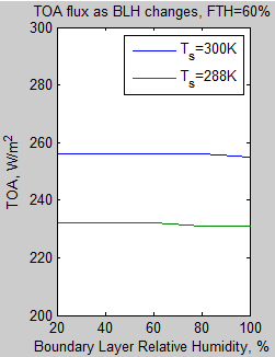
Figure 1

Is this surprising?

Now the downward longwave radiation (DLR) at the surface with the same conditions:

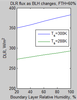
Figure 2

I could plot some more comparisons with different FTH values, but regardless of the FTH value the graphs of TOA flux vs BLH have the same characteristics.

Why, if water vapor is such a strong GHG, does the top of atmosphere radiation stay almost the same for a boundary layer almost dry through to completely saturated?

The reason is simple. The surface is emitting a blackbody radiation spectrum for that surface temperature (see note 2 in Part Two). The boundary layer is at almost the same temperature as the surface (2-3K difference in this case) so at a given wavelength radiation either gets transmitted, or gets absorbed and re-emitted (usually a combination). But if re-emitted, it is at almost the same temperature as the surface.

The radiative transfer equations show us that the change in flux as radiation travels through a body is caused by the difference between the temperature of the source of the radiation and the temperature of the body in question. This is explained a little more in Part Two and is an essential point to grasp.

So the upward radiation at TOA is the almost the same whether the boundary layer is saturated or dry.

But the surface DLR experiences a big difference as the boundary layer moisture changes. The reason why should be obvious by now, but this subject is quite difficult to take in when you are new to it.

What downward radiation is incident on the boundary layer from above? The answer is – nothing like as much as is incident on the boundary layer from below. The downward atmospheric radiation on this boundary layer is just the emission from the various GHGs (water vapor, CO2, O3, etc) and the water vapor concentration above is quite a lot lower than the boundary layer.

When the boundary layer is saturated with water vapor it emits very strongly across many bands. So the humidity of the boundary layer has a big impact on the DLR, but very little on the TOA outgoing radiation.

Free Tropospheric Humidity

Now let’s see the TOA changes as free tropospheric humidity, FTH, is changed – with BLH fixed at 100%:

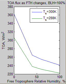
Figure 3

So now as the atmosphere above the boundary layer gets more water vapor it absorbs (and re-emits) more strongly. But the re-emission is from colder layers of the atmosphere so as this GHG increases in concentration up through the atmosphere, the TOA radiation reduces significantly. And if we reduce the outgoing radiation from the planet then, all other things being equal, the planet warms.

Let’s see the reasons a little more clearly, for the extreme case when we change FTH from 100% to 0%, with Ts=300K. The left side has the spectra for selected heights for both cases, and the right side has the difference between the two cases (at the same heights):

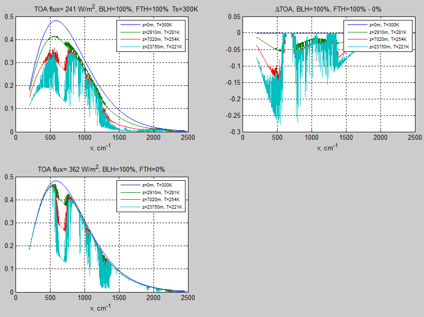
Figure 4 – Click to enlarge

[Note the title on the top right is slightly incorrect. It is not ΔTOA, it is the Δ (difference) at a few different heights including TOA.]

We can see that in the center of the CO2 band (600-700 cm^-1) there is zero change between the two cases at all heights – as expected.

The differences between the two cases occur:

strongly around 200-550 cm^-1 (50-18 μm) where water vapor absorption is quite strong
somewhat around the “atmospheric window” – which still absorbs due to the continuum, especially at the high water vapor saturation pressure when the surface temperature is near 300K
strongly around the 1500 cm^-1 (7μm) region where there are lots of water vapor absorption lines – however the surface emission is not so high in the first place so the overall effect is reduced

Now let’s look at DLR at the surface:

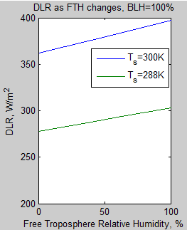
Figure 5

Even though the boundary layer is saturated, changes in water vapor above this layer still have a significant impact on the surface DLR.

Let’s see why by comparing the spectra of the 100% and 0% cases at 300K:

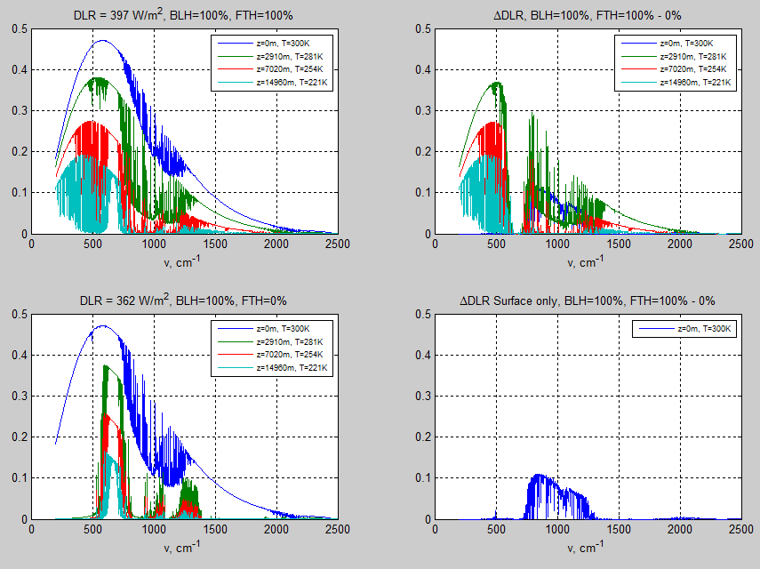
Figure 6 – Click to enlarge

The dark blue curve is the one we are measuring at the surface. The top right is the difference between the two cases at four different heights. The bottom right shows only the difference in spectra at the surface (it is hard to see it in the top right graph).

What is clear is that the difference is caused by the “mid-strength” absorbing/emitting “atmospheric window around 800-1200 cm^-1. The “background” DLR from the very top of atmosphere is of course zero (see figure 6 in Part Two). So anything that adds to the DLR on the way down assists the surface spectra.

This is not the case for very strongly emitting regions – see the region around 500 cm^-1. The boundary layer emits and absorbs due to water vapor so strongly in this wavenumber region that incident radiation from above is irrelevant to the surface measurement.

With and Without Water Vapor

Now let’s look at the upward spectra at various heights with (saturated) and without (dry) water vapor:

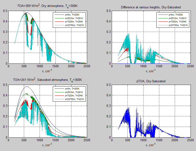
Figure 7 – Click to enlarge

The bottom right graph is just the top layer in the top right graph shown separately for clarity.

Conclusion

Most people’s untrained intuition about how different radiatively-active gases (=”greenhouse” gases) in different concentrations at different locations change the interaction of radiation with the atmosphere are wrong. Intuition needs to be informed by measurement and theory. It’s just not an intuitive subject.

We’ve seen that water vapor can have very different effects on TOA radiation and the surface. And we’ve seen that water vapor in different places has very different effects. Also we’ve seen the difference between a dry and saturated atmosphere.

Three important points:

1. On a technical note – this model has at least one important flaw, which is to do with how absorption lines change near the top of the troposphere – the Voigt profile vs the Lorenzian profile.

The Voigt profile is not yet implemented because when I last looked at it it made my head hurt trying to implement it in a useful manner (my attempt at the Voigt profile turned a surprisingly fast model given the 287,000 lines calculated in each of 10 layers into a bucket of sludge).

I am going to have another crack at this headache-inducing puzzle before trying to do lots of “what happens when CO2 concentrations are changed by small amounts” scenarios.

Actually, if there are any maths whizzes out there who would like to do the heavy lifting – or even just explain what seems simple to someone who has forgotten almost all maths ever learnt – please let me know here or via email at scienceofdoom – the usual bit – gmail.com. Probably you will get your name on the top of one of the graphs or something, no promises on the font size yet.

2. These scenarios we have seen are all from a “snapshot” of the climate in 1D without running it to a new equilibrium. Obviously if you change the water vapor from 0% to 100% the surface temperature won’t stay the same. Everything will change. When we have been comparing scenarios we have had mostly the exact same surface and atmospheric temperature. This is for a good reason. Small steps first. Actually, grasping atmospheric radiative transfer is a big step.

3. Changes in water vapor affect not just radiative transfer but latent heat and convection. The deep convection that “cranks the engine” on the important tropical circulation is from solar heating over the warmest oceans (see Clouds & Water Vapor – Part Five – Back of the envelope calcs from Pierrehumbert). Radiative transfer is just one piece of the puzzle.

Related Articles

Part One – some background and basics

Part Two – some early results from a model with absorption and emission from basic physics and the HITRAN database

Part Three – Average Height of Emission – the complex subject of where the TOA radiation originated from, what is the “Average Height of Emission” and other questions

Part Five – The Code – code can be downloaded, includes some notes on each release

Part Six – Technical on Line Shapes – absorption lines get thineer as we move up through the atmosphere..

Part Seven – CO2 increases – changes to TOA in flux and spectrum as CO2 concentration is increased

Part Eight – CO2 Under Pressure – how the line width reduces (as we go up through the atmosphere) and what impact that has on CO2 increases

Part Nine – Reaching Equilibrium – when we start from some arbitrary point, how the climate model brings us back to equilibrium (for that case), and how the energy moves through the system

Part Ten – “Back Radiation” – calculations and expectations for surface radiation as CO2 is increased

Part Eleven – Stratospheric Cooling – why the stratosphere is expected to cool as CO2 increases

Part Twelve – Heating Rates – heating rate (‘C/day) for various levels in the atmosphere – especially useful for comparisons with other models.

References

The data used to create these graphs comes from the HITRAN database.

The HITRAN 2008 molecular spectroscopic database, by L.S. Rothman et al, Journal of Quantitative Spectroscopy & Radiative Transfer (2009)

The HITRAN 2004 molecular spectroscopic database, by L.S. Rothman et al., Journal of Quantitative Spectroscopy & Radiative Transfer (2005)

Posted in Atmospheric Physics | 26 Comments

26 Responses

on January 9, 2013 at 7:13 pm | Reply clivebest

First let me ask a dumb question:

Why is it the case that ?

“The water vapor continuum absorbs as a function of the square of the number of water vapor molecules”

and which wavelengths cover this continuum ?

Basically (I think) your result is that the overall greenhouse effect of water vapor depends mainly on the relative humidity in the FTH – which I take as meaning roughly from about 1km altitude and above. Are there any long term measurements of relative humidity above 1 km? If so have they changed over the past 40 years ?

The boundary level directly effects net IR cooling from the surface. In addition to your clear evidence that DLR increases with relative humidity in the boundary layer, so low clouds also must offset incident solar radiation somewhat. My gut feeling “guess” is that during the day the net balance between the two is that cloud induced increase in albedo wins out over DLR. However during the night, humidity + low clouds block radiative heat loss from the surface leading to higher effective surface temperatures.

So IMHO, we are back to the basic question of climate science. How will H2O react to an increase in CO2 “radiative forcing” ?

I suspect only measurements will resolve this – not theory.
- on January 9, 2013 at 9:16 pm | Reply scienceofdoom
  
  Clive,
  
  A quick answer to your first question – it’s not a dumb question.
  
  “No one knows”. Or some know but everyone else is yet to agree.
  
  There are some theories.
  
  Because there are theories that are still competing for acceptance the solution is measurement and empirical fits – but measurements are needed through long paths and this is challenging.
  
  Grant Petty, A First Course in Atmospheric Radiation, says:
  
  There is significant continuum absorption by water vapor between the major absorption bands in the infrared and microwave bands. The physical mechanism behind the water vapor continuum remains a matter of some controversy. There are basically two competing theories:
  
  Far wings of the lines..
  
  H2O clusters..
  
  Keith Shine et al, The Water Vapour Continuum: Brief History and Recent
  Developments, Surveys in Geophysics (2012):
  
  Abstract:
  
  The water vapour continuum is characterised by absorption that varies smoothly with wavelength, from the visible to the microwave. It is present within the rotational and vibrational–rotational bands of water vapour, which consist of large numbers of narrow spectral lines, and in the many ‘windows’ between these bands.
  
  The continuum absorption in the window regions is of particular importance for the Earth’s radiation budget and for remote-sensing techniques that exploit these windows. Historically, most attention has focused on the 8–12 μm (mid-infrared) atmospheric window, where the continuum is relatively well-characterised, but there have been many fewer measurements within bands and in other window regions.
  
  In addition, the causes of the continuum remain a subject of controversy. This paper provides a brief historical overview of the development of understanding of the continuum and then reviews recent developments, with a focus on the near-infrared spectral region. Recent laboratory measurements in near infrared windows, which reveal absorption typically an order of magnitude stronger than in widely used continuum models, are shown to have important consequences for remote sensing techniques that use these windows for retrieving cloud properties.
  
  A few extracts from the paper:
  
  In addition to the absorption due to the individual spectral lines, water vapour possesses a slowly varying component of absorption, known as the continuum, which pervades both the bands and the windows from the visible through the infrared to the microwave. The absorption due to the water vapour spectral lines within the bands is normally so strong that the continuum in these regions is of secondary importance to the radiation budget (although, as will be discussed, it has turned out to be very important for understanding the causes of the continuum); in the windows, by contrast, the continuum is often the dominant cause of wavelength-averaged absorption (at least in clear skies) and so is of much greater importance both for the radiation budget and for remote-sensing techniques..
  
  ..Between 1970 and 1980, a number of experimental papers confirmed both the quadratic pressure dependence and strong negative temperature dependence of the water vapour self continuum…
  
  ..The failure of the Lorentzian line shape to predict the magnitude, temperature and pressure dependence of the water vapour continuum absorption contributed to the popularity of the dimer hypothesis. On the other hand, as noted above, it had long been recognised that the Lorentzian line shape is rather simplistic in its origin and that it might be expected to fail in modelling very far wings of absorption lines. New models of the line profile, especially far from the line centre, started to appear (see e.g., the discussion in Goody and Yung 1989). An integral representation of the absorption coefficient of spectral lines, developed earlier by adopting a quantum-mechanical formalism in the works of Anderson (1949) and Tsao and Curnutte (1962), was applied to specifically develop a far-wing approximation within a statistical approach in Fomin and Tvorogov (1973). Tvorogov and Nesmelova (1976) suggested an alternative far-wing model based on the semi-classical asymptotic approach, fully developed later by Nesmelova et al. (1986). In general, theoretical far-wing models of the continuum developed in that period were characterised by a number of adjustable parameters fit to experimental data, which, however, did not always guarantee that they would agree with experimental data at different temperatures or wavenumbers..
  
  ..Clough et al. (1980, 1989) demonstrated that the use of the Lorentz line approximation to represent the absorption in the far wings of the water vapour lines led to an overestimate of the strength of the continuum in the mid-infrared window and to a significant underestimate within water vapour bands; Varanasi and Chudamani (1987) noted the overestimate in the mid-infrared region, although the extent of the overestimate depends on the assumed vapour and air pressures and temperature. The parameterisation used in the CKD model was very successful compared to all previous empirical and theoretical models and became the ‘industry standard’ in radiation codes within the atmospheric sciences…
  
  ..The dimer explanation of the continuum also underwent further development during this period. The dimer hypothesis was largely supported at the time by a single characteristic of the observations—the negative temperature dependence. Hinderling et al. (1987) presented a comprehensive laboratory study of the mid-infrared continuum based on laser photoacoustic spectroscopy. Their measurements of the temperature dependence of the continuum between -20C and +70C were consistent, but not conclusively so, with a dimer interpretation for absorption. They also performed an analysis of absorption in supersaturated air in a diffusion chamber. They inferred that the absorption cross-section for the dimer was about 30 times smaller than was required to explain the observed continuum absorption and concluded that the mid-infrared continuum was predominantly due to local absorption lines and far wings of distant lines. However, their inference appears to be based on a somewhat arbitrary separation of the observed absorption between dimers and far wings at one position in their chamber, and a different separation could have led them to a quite different conclusion..
  
  ..In 2003, a major new version of CKD continuum model was issued, which represented the first recomputation of the entire self and foreign continua since the original CKD model was developed in the 1980s. The new model, called MT_CKD (the MT standing for two of the originators of the new version—Mlawer and Tobin—see Mlawer et al. (2012) and Delamere et al. (2010)), is based on an updated formulation and has been widely adopted within the atmospheric science community.
  
  ..Vigasin (2000) suggested a simple parameterisation of continuum absorption in the mid-infrared and microwave spectral regions using just a few physical parameters related to the water complexes. He has shown that this model is in a good agreement with known measurements.
  
  And if you look in Google Scholar for water vapor continuum you will find plenty of papers, most quite inaccessible of course.
  - on January 9, 2013 at 9:53 pm Pekka Pirilä
    
    .. and I thought that it’s obvious. It turns out from those papers that what I thought as obvious is only one of the theories.
    
    What I had in mind is clustering. Water molecules are known to stick together by hydrogen bridge. That would lead to short lived clusters of two molecules and occasionally even more than two. It’s natural for such a cluster to have a continuum spectrum as both molecules can contribute to emission and absorption. The number of such clusters would also grow with the density of water molecules making the square law natural.
    
    As this idea is evidently not uncontroversial the case must be that it has not been possible to understand quantitatively the continuum through this explanation. A plausible explanation is only a hypothesis until it has been found to lead to quantitatively right results through well justified calculations. There must be problems on this level.
  - on January 10, 2013 at 12:03 am DeWitt Payne
    
    My candidate is collision induced absorption, self and foreign. See for example:
    
    Click to access mlawer_ej.pdf
    
    It’s relatively easy to calculate the CIA spectrum for symmetrical diatomic molecules like N2 and O2, but that absorption is many orders of magnitude weaker than for water vapor and is only important for limb paths in the upper atmosphere where there isn’t any water vapor to speak of and for very cold atmospheres like that of Titan where the absorption peak at ~100 cm-1 is near the thermal emission peak. Water vapor, being an asymmetric molecule, is much more difficult to calculate.
  - on January 10, 2013 at 7:17 am Pekka Pirilä
    
    Actually my intuitive feeling is that all the three different mechanisms that I see discussed heavily in recent literature are different aspects of “water molecules sticking together”.
    
    Dimer-theory discusses properties of a “supermolecule” of two H2O molecules held together by the hydrogen bond for extensive periods (on molecular scale) and how the two mole oscillate with respect to each other and rotate as a pair. This explains continuum in the at longest wavelengths, but not at the most important ones from the point of view of atmospheric heat transfer.
    
    The other two theories must also explain, why water is different from other molecules. CIA requires that the two colliding molecules stay together longer when they collide and the same may be true also for far-wing theory although I have right now less understanding of that. The role of the hydrogen bond is not as straightforward for these mechanisms as for dimers but I think that it’s essential again. The molecule pairs responsible for these other two mechanisms are not as long-lived as dimers but still longer-lived than the periods that other molecular pairs stay together in collisions.
    
    The basic idea that molecules stick together seems essentially required by the Heisenberg uncertainty principle to explain continuum spectra. This is the basis for my intuition, but as I wrote in my previous message, a hypothesis based on such generic arguments is only a hypothesis until a more detailed understanding capable of producing quantitative predictions is reached.
  - on January 10, 2013 at 10:19 am Pekka Pirilä
    
    I hadn’t read the Shine et al paper although I downloaded it some time ago.
    
    Having now read the Chapter 2 I see that it fits well with my intuition while it’s certainly much more detailed and justified. The authors seem to consider the role of dimers to be significant at all IR wavelengths when also short lived dimers are taken into account:
    
    The experimental work also indicated some broad spectral features that could not be explained by the theoretical dimer spectra. Recently, Ptashnik et al. (2011a) suggested that this could be explained by the fact that the theoretical spectra accounted only for truly bound dimers. In addition to these bound dimers, it was proposed by Vigasin (1985, 1991, 2003, 2010) and Epifanov and Vigasin (1997), by a statistical partitioning of molecular pairs in phase space, that shorter-lived quasi-bound dimers should be of equal importance in atmospheric conditions. A simplified calculation (Ptashnik et al. 2011a) indicated that these quasi-bound dimers might explain the additional spectral features in the observed near-room temperature spectra of the continuum. This may also help to explain the wavelength variation of the temperature dependence of the continuum and non-exponential temperature dependence of the continuum at particular wavenumbers in the mid-infrared window detected by Baranov et al. (2008). Classical- and quantum-mechanical calculations by Schenter et al. (2002) for H2O–H2O pairs and 3D classical trajectory simulations by Lokshtanov et al. (2005) provide independent support for the statistical partitioning approach of Vigasin and hence support the view that quasi-bound water dimers play an important role at close to room temperature. Ptashnik et al. (2011a) also reviewed the role of dimers in explaining the continuum in the mid- and far-infrared—bound dimers may contribute 15–40%, with an expected additional contribution from the quasi-bound dimers.
    
    They note, however,
    
    Given the uncertainties in the width and shape of the vibrational bands of the dimer, the situation in the windows, which is more important from an atmospheric radiation point of view, is less clear.
    
    ..
    
    These measurements, which are summarised in Fig. 3, are not inconsistent with the dimer explanation, but they are far from conclusive given the poor understanding of the shape and width of the dimer bands.
    
    One additional point is that the Lorentzian line-shape has so long wings that it may actually lead in some cases rather to an overestimate of continuum rather than an underestimate. As stated also by Shine et al, the Lorentzian line-shape is derived from the assumption of instantaneous interaction. A distance of 100 1/cm from the line center corresponds to a time of roughly 0.05 ps. During that time a gas molecule moves typically around 20 pm or 0.2 angstrom – and the unit of angstrom is just that of atomic dimension. Thus it’s obvious that the assumption of instantaneous collisions fails at intervals much less than 1 ps, and the Lorentzian line-shape is not justified anymore at distances approaching 100 1/s from the line center.
  - on January 11, 2013 at 1:29 pm clivebest
    
    Thanks for all the comments. So, If I understand correctly hydrogen bonds can develop between molecules during collisions of molecules in water vapor and emit over a broad IR spectrum range. The probability of this occurring increases with concentration. In addition the total number of molecules available to “cluster” also increases with concentration. This way you can get a picture of how total absorption could go as the square of concentration.
- on January 10, 2013 at 10:17 am | Reply scienceofdoom
  
  Clive,
  
  ..Basically (I think) your result is that the overall greenhouse effect of water vapor depends mainly on the relative humidity in the FTH – which I take as meaning roughly from about 1km altitude and above. Are there any long term measurements of relative humidity above 1 km? If so have they changed over the past 40 years ?
  
  Not particularly good ones.
  
  I wrote about water vapor trends in Water Vapor Trends and Part Two.
  
  Those two articles should give you some background on the measurement issues in decadal trends and especially in the upper troposphere. I listed lots of papers worth reading.
on January 10, 2013 at 1:27 am | Reply DeWitt Payne

SoD,

There is a MATLAB wrapper for LBLRTM. That doesn’t help me because I don’t have MATLAB, but it might help you.
on January 13, 2013 at 4:59 am | Reply Visualizing Atmospheric Radiation – Part Seven – CO2 increases « The Science of Doom

[…] a look at Part Three – Average Height of Emission and Part Four – Water Vapor for more […]
on January 23, 2013 at 9:39 am | Reply Visualizing Atmospheric Radiation – Part Ten – “Back Radiation” « The Science of Doom

[…] take a look. Note that Part Four – Water Vapor already has some graphs of how the DLR or “back radiation” changes with water vapor […]
on February 2, 2013 at 7:43 am | Reply Visualizing Atmospheric Radiation – Part Six – Technical on Line Shapes « The Science of Doom

[…] Part Four – Water Vapor – results of surface (downward) radiation and upward radiation at TOA as water vapor is changed […]
on February 2, 2013 at 7:45 am | Reply Visualizing Atmospheric Radiation – Part Five – The Code « The Science of Doom

[…] Visualizing Atmospheric Radiation – Part Four – Water Vapor Visualizing Atmospheric Radiation – Part Six – Technical on Line Shapes […]
on February 2, 2013 at 7:48 am | Reply Visualizing Atmospheric Radiation – Part Three – Average Height of Emission « The Science of Doom

[…] Visualizing Atmospheric Radiation – Part Two Visualizing Atmospheric Radiation – Part Four – Water Vapor […]
on February 2, 2013 at 7:51 am | Reply Visualizing Atmospheric Radiation – Part One « The Science of Doom

[…] Part Four – Water Vapor – results of surface (downward) radiation and upward radiation at TOA as water vapor is changed […]
on February 2, 2013 at 7:53 am | Reply Visualizing Atmospheric Radiation – Part Eight – CO2 Under Pressure « The Science of Doom

[…] Part Four – Water Vapor – results of surface (downward) radiation and upward radiation at TOA as water vapor is changed […]
on February 12, 2013 at 1:17 pm | Reply Clouds & Water Vapor – Part Seven – Upper Tropospheric Models & Measurement « The Science of Doom

[…] The upper troposphere is very dry, and so the mass of water vapor we need to change OLR by a given W/m² is small by comparison with the mass of water vapor we need to effect the same change in or near the boundary layer (i.e., near to the earth’s surface). See also Visualizing Atmospheric Radiation – Part Four – Water Vapor. […]
on August 12, 2013 at 6:29 pm | Reply Over 4.5 Billion to die by 2012 - Page 11 - US Message Board - Political Discussion Forum

[…] No, they don't. They cover the SAME spectrums. Here's what science says about this debate. Visualizing Atmospheric Radiation ? Part Four ? Water Vapor | The Science of Doom Of course, only people interested in science will read it, and only people educated in science […]
on March 12, 2014 at 3:33 pm | Reply Nobodyknows

What is water vapor?
I came across a very interesting site on water (Martin Chaplin). As I understand it, there are various conditions of water vapor which has different radiation characteristics. Most of the water is undercooled. In the very highest layer of tropsfæren it is ice or water glass that absorbs and spreads long wave radiation in a peculiar way. One would think that this influences the radiation from the atmosphere. I have not seen that this theme have been adressed.
http://www1.lsbu.ac.uk/water/vibrat.html
on September 9, 2017 at 6:44 pm | Reply Brad Schrag

Trying to understand figures 1 and 2 better. I realize this isn’t the place for intuition but mine says that as the humidity increases there is an increase in the total amount of radiation. Since ToA remains almost constant but there is a drastic uptick in DLR with the humidity change. Having trouble grasping an increase in DLR without an equivalent decrease in ToA if anyone help or direct me where to look. Thanks.
- on September 9, 2017 at 8:09 pm | Reply scienceofdoom
  
  Brad,
  
  It’s a good question, once you have clarity on the answer, a lot more about atmospheric radiation makes sense.
  
  Picture the atmosphere with no CO2, or methane, or water vapor. We look up in the sky (from the surface) with our longwave radiation detector (4-100um). What do we measure? Zero (just about).
  
  This is because the atmosphere is not absorbing and therefore not emitting any radiation.
  
  Now we get our satellite with our longwave radiation detector to look down at the surface, say somewhere with a temperature around 15’C (288K). What do we measure? About 390W/m².
  
  Hopefully those two points make sense. Now we add a lot of water vapor in the boundary layer (bottom km or so of the atmosphere).
  
  Now we have gone from a transparent atmosphere (which doesn’t emit) to one that does. So we are going to measure significant DLR.
  
  But the satellite is now measuring some radiation from the surface that made it through, and some radiation from the bottom 1km of the atmosphere that is around 0-6K cooler. A mix. Overall the atmosphere is close to the surface temperature so it will reduce the OLR a little but not much.
  
  Do these points make sense?
  - on September 9, 2017 at 9:16 pm Brad Schrag
    
    It maybe just clicked. Adding in the boundary layer has simply added in more mass that, at the given temperature, is going to emit just the same and cumulatively increase the amount of LR. The amount of surface radiation that it’s absorbing and emitting back to the surface is simply offset by its own production of OLR, which is why there isn’t seen as much of a decrease with humidity. How’s that sound?
  - on September 9, 2017 at 10:14 pm Brad Schrag
    
    Rereading my interpretation I realize that it maybe seems unclear.
    
    Up until now, the visualizing of the atmosphere has focused on how co2 has mostly interacted with emissions produced at the surface (or maybe it hasn’t and I’ve just been visualizing things wrong). So when I see figure 1 remain mostly flat, while figure 2 increases I was wondering where this extra radiation was coming from. Since I was only picturing the surface as a place of origin for the radiation it didn’t mask sense that there could be an increase in DLR without a subsequent decrease in ToA.
    
    Reading your response I had the idea of removing the surface entirely from the equation, that is to just have a hollow, floating sphere at 15C of humidity. From the satellites perspective it’s going to still be picking up OLR from the blob of humidity. Then adding the surface back in, there is going to be some extra OLR that makes it through from the surface, DLR produced from the humidity directed at the surface, as well as absorption and re emission happening due to water vapor. All to the cumulative effect of no change at ToA, but a sizeable increase at surface level.
  - on September 10, 2017 at 6:47 am scienceofdoom
    
    When person A tries to explain their conceptual ideas about how radiation works it’s never clear whether person B has understood person A’s ideas or not.
    
    I think you still have OLR slightly wrong, but that could just be my misreading of your explanation. So if this helps, good. And if it doesn’t help, I might just have misunderstood your explanation.
    
    If the surface is a black body, it is already a perfect emitter. So adding lots of water vapor at, say, 1km above the surface doesn’t “add” to the OLR.
    
    In fact what it does is reduce OLR.
    
    Imagine so much water vapor that it is in fact a black body floating 1km above the surface. The temperature of this water vapor is 6K lower than the surface temperature. And this water vapor is a black body.
    
    All radiation from the surface is absorbed by this water vapor (because it is a perfect absorber). So no surface radiation is transmitted into space. It’s absorbed by the water vapor.
    
    Therefore, the emission to space is only from the water vapor. And the water vapor is cooler than the surface. So OLR is reduced.
    
    Does this make sense? Maybe it makes sense and doesn’t answer your question.
- on September 10, 2017 at 8:48 am | Reply Frank
  
  Brad: If you are interested, you can go the website below and easily use MODTRAN to predict what the emission from highly simplified atmospheres would look like.
  
  http://climatemodels.uchicago.edu/modtran/
  - on September 10, 2017 at 12:26 pm Brad Schrag
    
    Frank,
    Thanks.
    
    And SoD,
    Yes. Does sound like I’m on the right trackbut you explain it much better than I.

Comments RSS

	Planet TX on Ghosts of Climates Past
	Les subtilités de l… on CO2 – An Insignificant T…
	Natural Variability,… on Models, On – and Off – the Cat…
	Natural Variability,… on Models, On – and Off – the Cat…
	Natural Variability,… on Opinions and Perspectives – 6…
	bobhisey on Natural Variability, Attributi…
	Windchaser on Natural Variability, Attributi…
	bobhisey on Natural Variability, Attributi…
	Windchaser on Natural Variability, Attributi…
	bobhisey on Natural Variability, Attributi…
	Windchaser on Natural Variability, Attributi…
	bobhisey on Natural Variability, Attributi…
	Dodo on Natural Variability, Attributi…
	Windchaser on Natural Variability, Attributi…
	Dredd on Natural Variability, Attributi…

The Science of Doom

Evaluating and Explaining Climate Science