Understanding atmospheric radiation is not so simple. But now we have a line by line model of absorption and emission of radiation in the atmosphere we can do some “experiments”. See Part Two and Part Five – The Code.
Many people think that models are some kind of sham and climate scientists should be out there doing real experiments. Well, models aren’t a sham and climate scientist are out there doing lots of experiments. Various articles on Science of Doom have outlined some of the very detailed experiments that have been done by atmospheric physicists, aka climate scientists.
When you want to understand why some aspect of a climate mechanism works the way it does, or what happens if something changes then usually you have to resort to a mathematical model of that part of the climate.
You can’t suddenly increase the amount of a major GHG across the planet, or slow down the planetary rotation to ½ its normal speed. Well, not without a sizable investment, a health and safety risk, possible inconvenience to a lot of people and, at some stage, awkward government investigations.
You can’t stop the atmosphere emitting radiation or test a stratosphere that gets cooler with height. But you can attempt to model it.
Mathematical models all have their limitations. We have to understand what the model can tell us and what it can’t tell us. We have to understand what presuppositions are built into the model and what can change in real life that is not being modeled in the maths. It’s all about context.
(Well-designed) models are not correct and are not incorrect. They are informative if we understand their limitations and capabilities.
In contrast to mathematical models built around the physics of climate mechanisms, many people commenting in the blog world (or even writing blogs) have a vague mental model of how climate works. This of course is way way ahead of a climate model built on physics. It has the advantage of not being written down in equations so that no one can challenge it and seemingly plausible hand-waving argument 1 can be traded against hand-waving argument 2. Unfortunately, on this blog we don’t have the luxury of those resources and – where experiments are not available or not possible – we will have to evaluate the results of mathematical models built on physics and observations.
All the above is not an endorsement of what GCMs tell us. And not an indictment. Hopefully no one reading the above paragraphs came to either conclusion.
When I first built the line by line model it had more limitations than today. One early problem was the stratosphere. In real life the temperature of the stratosphere increases with height. In the model the temperature decreased with height.
This was expected. O2 and O3 absorb solar radiation (primarily ultraviolet) and warm mainly the middle layers of the stratosphere. But the model didn’t have this physics. The model, at this stage, primarily modeled the absorption and emission of terrestrial (aka ‘longwave’) radiation by the atmosphere.
So, after a few versions a very crude model of solar absorption was added. Unfortunately, this solar absorption model still did not create a stratosphere that increased with temperature. This was quite disappointing.
Then commenter Uli pointed out that the model had too much stratospheric water vapor and I added a new parameter to the model which allowed stratospheric water vapor to be set differently from the free troposphere. (So far I’ve been using a realistic level of 6ppmv).
The result was happily that the stratosphere, left to its own (model) devices, started increasing with temperature. The starting point is simply a temperature profile dictated to the model, and the finish point is how the physics ends up calculating the final temperature profile:
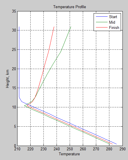
Figure 1 – A warmer stratosphere and a happier climate model
At the same time, I’ve been updating the model so that it can run to some kind of equilbrium and then various GHGs can be changed.
This was to calculate “radiative forcing” under various scenarios, and specifically I wanted to show how energy moved around in the climate system after a “bump” in something like CO2. This is something that many many people can’t get right in their heads. One of the objectives of the model is to show bit by bit how the increased CO2 causes a reduction in net outgoing radiation, and how that in turn pushes up the atmospheric and surface temperature.
On this journey, once the model stratosphere was behaving a little like its real-life big brother it occurred to me that maybe we could answer the question of why the stratosphere was expected to cool with increased CO2.
See Stratospheric Cooling for some background.
Previously I have worked under the assumption that there are lots of competing “terms” in the energy balance equation for how the stratosphere responds to more CO2 and so simple conceptual models are not going to help.
Now the Science of Doom Climate Model (SoDCM) comes to the rescue.
In fact, while I was waiting for lots of simulations to finish on the PC I was reading again the fascinating Radiative Forcing and Climate Response, by Hansen, Sato & Ruedy, JGR (1997) – free paper – and in a groundhog day experience realized I didn’t understand their flux graphs resulting from various GCM simulations. So the SoDCM allowed me to solve my own conceptual problems.
Maybe.
Let’s take a look at stratospheric cooling.
Understanding Flux Curves
In this simulation:
- CO2 at 280 ppm
- no ozone, CH4 or NO2 for longwave absorption
- boundary layer humidity at 80%
- free tropospheric humidity at 40%
- stratospheric water vapor at 6 ppmv
- tropopause at 200 hPa
- top of atmosphere (TOA) at 1 hPa
- solar radiation at 242 W/m² with some absorbed in the stratosphere and troposphere as shown in figure 1 of Part Nine – Reaching Equilibrium
The surface temperature reached equilibrium at 281K and the tropopause was at 11 km:
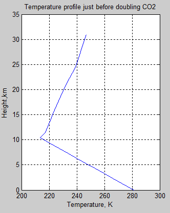
Figure 2
The equilibrium was reached by running the model for 500 (model) days, with timesteps of 2 hours. The ocean depth was only 5 meters simply to allow the model to get to equilibrium quicker (note 1).
Then at 500 days the CO2 concentration was doubled to 560 ppm and we capture a number of different values from the timestep before the increase and the timestep after the increase.
Let’s take a look at the up and down fluxes through the atmosphere. See also figure 6 of Part Two. In this case we can see pre- and post-2xCO2, but let’s first just try and understand what these flux vs height graphs actually mean:
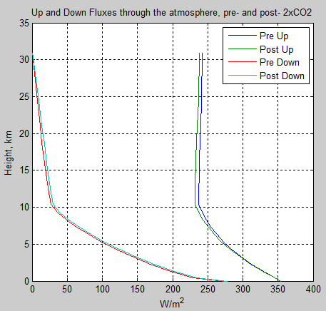
Figure 3 – Understanding the Basics
If flux just stays constant (vertical line) through a section of the atmosphere what does it mean?
It means there is no net absorption. It could mean that the atmosphere is transparent to that radiation. It could mean that the atmosphere emits exactly the same amount that it absorbs. Or some of both. Either way, no change = no net radiation absorbed.
Take a look in figure 3 at the (pre-CO2 doubling) upward flux above 10km (in the stratosphere). About 237 W/m² enters the bottom of the stratosphere and about 242 W/m² leaves the top of atmosphere. So the stratosphere is 5 W/m² worse off and from the first law of thermodynamics this either cools the stratosphere or something else is supplying this energy.
Now take a look at the (pre-CO2) downward flux in the stratosphere. At the top of atmosphere there is no downward longwave radiation because there is no source of this radiation outside of the atmosphere. So downward flux = 0 at TOA.
At the bottom of the stratosphere, about 27 W/m² is leaving. So zero is entering and 27 W/m² is leaving – this means that the stratosphere is worse off by 27 W/m².
If we add up the upward and downward longwave fluxes through the stratosphere we find that there is a net loss of about 32 W/m². This means that if the stratosphere is in equilibrium some other source must be supplying 32 W/m².
In this case it is the solar absorption of radiation.
If we were considering the troposphere it would most likely be convection from the surface or lower atmosphere that would be balancing any net radiation loss from higher up in the troposphere.
So, to recap:
- think about the direction radiation is travelling in:
- if it is reducing in the direction it is travelling then energy is absorbed into that section of the atmosphere
- if it is increasing in the direction it is travelling then energy is being lost from that section of the atmosphere
- if plots of flux against height are vertical that means there is no change in energy in that region
- if flux vs height is constant (vertical) then it either means
- the atmosphere is transparent to that radiation, OR
- the atmosphere is isothermal in that region (emission is balanced by absorption)
Take another look at figure 3 below 10km:
- The upward radiation is reducing with height – energy is absorbed by each level of the atmosphere. This is a net heating.
- The downward radiation is increasing – energy is lost from each level of the atmosphere. This is a net cooling.
- The slope of the curves is not equal. This is because energy is transferred via convection in the troposphere.
Understanding these concepts is essential to understanding radiation in the atmosphere.
Upward Flux from Changes in CO2
Let’s take a closer look at the upward and downward changes due to doubling CO2. So the “pre” curve is the atmosphere in a nice equilibrium condition. And the “post” curve is immediately after CO2 has been doubled, long before any equilibrium has been reached.
Let’s zoom in on the upward fluxes in the stratosphere pre- and immediately post-CO2 doubling:
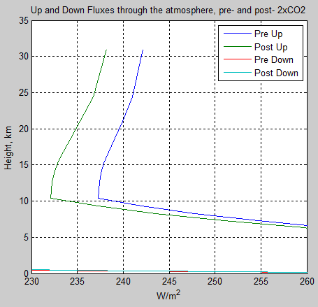
Figure 4
Even though the curves are roughly parallel from 10km through to 30km you should be able to see that there is a larger gradient on the post-2xCO2 curve. So pre-CO2 increase, the stratosphere loses a net upward of about 5 W/m², and after CO2 increase the stratosphere loses a net upward of about 6 W/m².
This means more CO2 increases the cooling of the stratosphere when we consider the upward flux. So now the question is, WHY?
If we want to understand the answer, the most useful ingredient is to look at the spectral characteristics of pre- and post. Here we take the radiation leaving at TOA and subtract the radiation entering at the tropopause. So we are considering the net energy lost (why lost? because this calculation is energy out – energy in), and as a function of wavenumber.
Here is the spectral graph of energy lost by the stratosphere due to upwards radiation, before the CO2 increase:
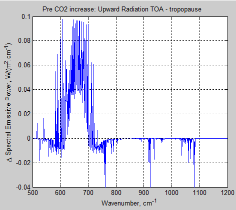
Figure 5
The post-CO2 doubling looks very similar so here is a comparison graph, with a slight smoothing (moving average window) just to allow us to see a little more clearly the main differences:
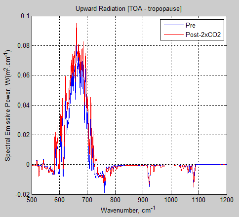
Figure 6
So we see that in the case of post-2xCO2, the energy lost is a little higher, and it is in the wavenumber region where CO2 emits strongly. CO2’s peak absorption/emission is at 667 cm-1 (15 μm).
Just to confirm, here is the difference – post-2xCO2 minus pre-2xCO2 and not smoothed:
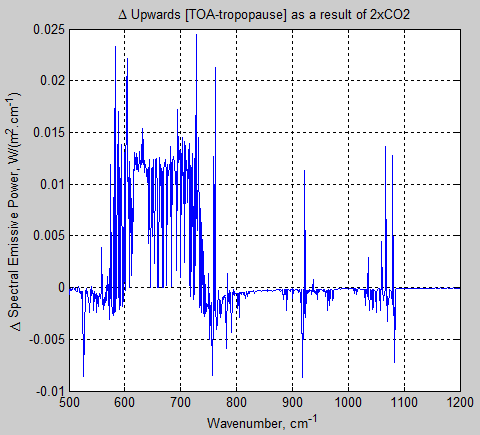
Figure 7
We can see that the main regions of CO2 absorption and emission are the reason. And we note that the temperature of the stratosphere is increasing with height.
So the reason is clear – due to principles outlined earlier in Part Two. Because the stratospheric temperature increases with height, the net emission (i.e., emission less absorption) of radiation, as we go up through the stratosphere will be a progressively higher value. And once we increase the amount of CO2, this net emission will increase even further.
This is what we see in the spectral intensity – the net change in stratospheric emission [(out-in)2xCO2 – (out-in)1xCO2] increases due to the emission in the main CO2 bands.
Downward Flux from Changes in CO2
Here is what we see when we zoom in on the downward flux in the stratosphere:
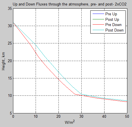
Figure 8
Of course, as already mentioned, the downward longwave flux at TOA must be zero.
This time it is conceptually easier to understand the change from more CO2. There’s one little fly in the understanding ointment, but let’s come to that later.
So when we think about the cooling of the stratosphere from downward flux it’s quite easy. Coming in at the top is zero. Coming out of the bottom (pre-CO2 increase) is about 27 W/m². Coming out of the bottom (post-2xCO2) is about 30 W/m². So increasing CO2 causes a cooling of about 3 W/m² due to changes in downward flux.
Here is the spectral flux (unsmoothed) downward out of the bottom of the tropopause, pre- and post-2xCO2:
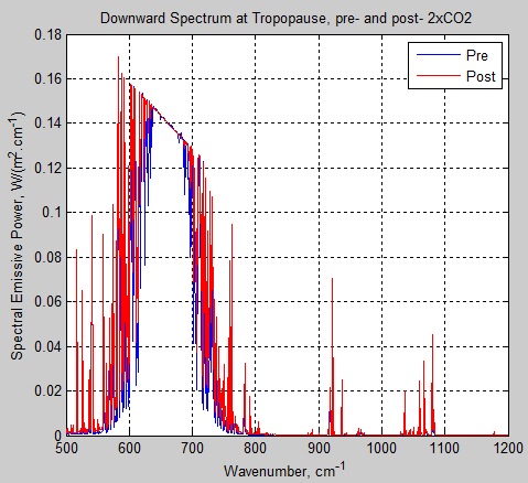
Figure 9
And as with figure 7, below is the difference in downward intensity as a result of 2xCO2. This is post less pre, so the positive value overall means a cooling – as we saw in the total flux change in figure 8.
The cause is still due to the CO2 band but the specifics are a little different from the upward change. Here the center of the CO2 band has zero effect. But the “wings” of the CO2 band – around 600 cm-1 and 700 cm-1 are the places causing the effect:
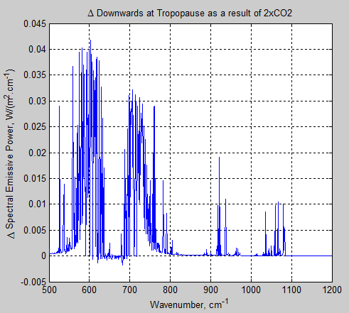
Figure 10
The temperature is reducing as we go downwards so the emission from the center of the CO2 band cannot be increasing as we go downward. If we look back at figure 7 for the upward direction, the temperature is increasing upward so the emission from the center of the CO2 band must be increasing.
And the conceptual fly in the ointment alluded to earlier – this one can be confusing (or simple..) – if the starting flux at TOA is zero and the temperature decreases downward surely the downward flux only gets less? Less than zero? Instead, think of the whole stratosphere as a body. It must emit radiation due to its temperature and emissivity. It can’t absorb any radiation from above (because there is none), so it must emit some downward radiation. As its emissivity increases with more GHGs it must emit more radiation into the troposphere. It’s simple really.
Let’s now finalize this story by considering the net change in flux with height due to CO2 increases. Here if “net” is increasing with height it means absorption or heating. And if “net” is reducing with height it means emission or cooling. See note 2 where the details are explained.
So the blue line (upward flux) decreasing from the tropopause up to TOA means that the change in flux is cooling the stratosphere. And likewise for the green line (downward flux). This is just the results already shown as spectral changes now shown as flux changes:
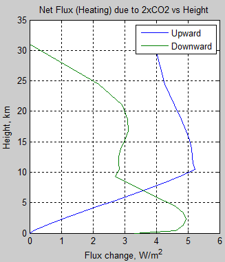
Figure 11
Net Effect
If we combine figure 11 for the total net effect of doubling CO2:
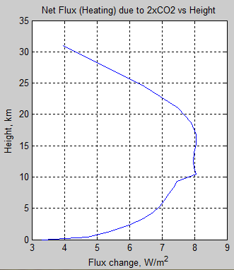
Figure 12
From the tropopause at 11km through to TOA we can see that the combined change in flux due to CO2 doubling causes a cooling of the stratosphere. (And from the surface up to the tropopause we see a heating of the troposphere).
By comparison, here is an extract from Hansen et al (1997):
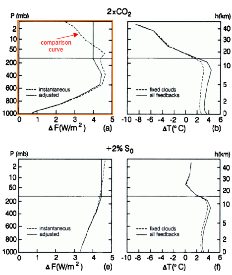
From Hansen et al (1997)
Figure 13
The highlighted instantaneous graph is the one for comparison with figure 12.
This is the case before the stratosphere has relaxed into equilibrium. Note that the “adjusted” graph – stratospheric equilibrium – has a vertical line for ΔF vs height, which simply means that the stratosphere is, in that case, in radiative equilibrium.
Notice as well that the magnitude of my graph is a lot higher. There may be a lot of reasons for that, including that fact that mine is one specific case rather than some climatic mean, and also that the absorption of solar radiation in my model has been treated very crudely. (Lots of other factors include missing GHGs like CH4, N2O, etc).
Reasons
So we have seen that the net emission of radiation by CO2 bands is what causes the cooling from upward radiation and the cooling from downward radiation when CO2 is increased.
For further insight, I amended the model so that on the timestep before and just after equilibrium the stratosphere was:
A) snapped back to an isothermal case, with the temperature set at the tropopause temperature just calculated
B) forced into a cooling at 4 K/km (c.f. the troposphere with a lapse rate of 6.5 K/km)
Case A, temperature profile just before and after equilibrium:
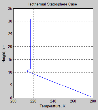
Figure 14
And the comparison to figure 11:
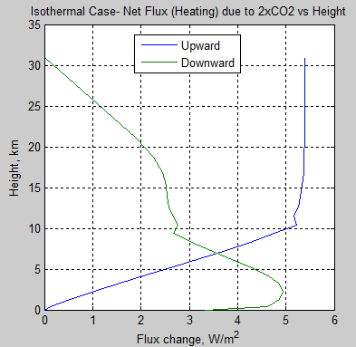
Figure 15
We can see that the downward flux change is similar to figure 11, but the upward flux is different. It is fairly constant through the stratosphere. This is not surprising. The flux from below is either transmitted straight through, or is absorbed and re-emitted at the same temperature. So no change to upward flux.
But the downward flux only results from the emission from the stratosphere (nothing transmitted through from above). As CO2 is increased the emissivity of the atmosphere increases and so emission of radiation from the stratosphere increases. The fact that the stratospheric temperature is isothermal has a small effect as can be seen by comparing the green curve on figures 15 & 11. But it isn’t very significant.
Now let’s consider case B. First the temperature profile:
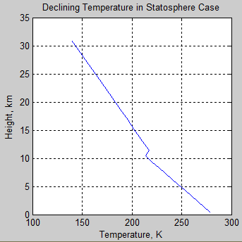
Figure 16
Now the net flux graph:
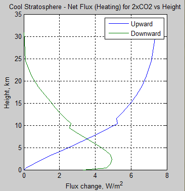
Figure 17
Here we see that the effect of increased CO2 on the upward flux is now a heating in the stratosphere. And the net change in downward flux still has a cooling effect.
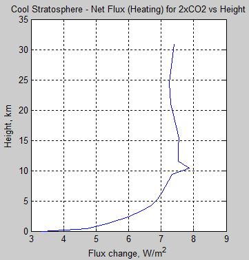
Figure 18
Here we see that for a stratosphere where temperature reduces with altitude, doubling CO2 would not have a noticeable effect on the stratospheric temperature. Depending on the temperature profile (and other factors) there might be a slight cooling or a slight heating.
Conclusion
This is a subject where it’s easy to confuse readers – along with the article writer. Possibly no one that was unclear before made it the whole way and said “ok, got it”.
Hopefully, if you only made it only part of the way through, you now have a better grasp of some of the principles.
The reasons behind stratospheric cooling due to increased GHGs have been difficult to explain even for very knowledgeable atmospheric physicists (e.g., one of many).
I think I can explain stratospheric cooling under increasing CO2. I think I can see that other factors like the exact temperature profile of the stratosphere on any given day/month and the water vapor profile (not shown in this article) will also affect the change in stratospheric temperature from increasing CO2.
If the bewildering complexity of up/down, in-out, net of in-out, net of in-out for 2xCO2-original CO2 has left you baffled please feel free to ask questions. This is not an easy topic. I was baffled. I have 4 pages of notes with little graphs and have rewritten the equations in note 2 at least 5 times to try and get the meaning clear – and am still expecting someone to point out a sign error.
Related Articles
Part One – some background and basics
Part Two – some early results from a model with absorption and emission from basic physics and the HITRAN database
Part Three – Average Height of Emission – the complex subject of where the TOA radiation originated from, what is the “Average Height of Emission” and other questions
Part Four – Water Vapor – results of surface (downward) radiation and upward radiation at TOA as water vapor is changed
Part Five – The Code – code can be downloaded, includes some notes on each release
Part Six – Technical on Line Shapes – absorption lines get thineer as we move up through the atmosphere..
Part Seven – CO2 increases – changes to TOA in flux and spectrum as CO2 concentration is increased
Part Eight – CO2 Under Pressure – how the line width reduces (as we go up through the atmosphere) and what impact that has on CO2 increases
Part Nine – Reaching Equilibrium – when we start from some arbitrary point, how the climate model brings us back to equilibrium (for that case), and how the energy moves through the system
Part Ten – “Back Radiation” – calculations and expectations for surface radiation as CO2 is increased
Part Twelve – Heating Rates – heating rate (‘C/day) for various levels in the atmosphere – especially useful for comparisons with other models.
References
The data used to create these graphs comes from the HITRAN database.
The HITRAN 2008 molecular spectroscopic database, by L.S. Rothman et al, Journal of Quantitative Spectroscopy & Radiative Transfer (2009)
The HITRAN 2004 molecular spectroscopic database, by L.S. Rothman et al., Journal of Quantitative Spectroscopy & Radiative Transfer (2005)
Radiative Forcing and Climate Response, by Hansen, Sato & Ruedy, JGR (1997) – free paper
Notes
Note 1: The relative heat capacity of the ocean vs the atmosphere has a huge impact on the climate dynamics. But in this simulation we were interested in reaching an equilibrium for a given CO2 concentration & solar absorption – and then seeing what happened to radiative balance immediately after a bump in CO2 concentration.
For this requirement it isn’t so important to have the right ocean depth needed for decent dynamic modeling.
Note 2: The treatment of upward and downward flux can get bewildering. The easiest approach is to just consider the change in flux in the direction in which it is travelling. But because upward and downward are in opposite directions, F↑ is in the direction of z, and F↓ is in the opposite direction to z, so heating and cooling are in opposite directions.
Due to changing GHGs:
If F↑(z)2xCO2 – F↑(z) < 0 => Heating below height z (less flux escaping);
F↑(z)2xCO2 – F↑(z) > 0 => Cooling below height z
If F↓(z)2xCO2 – F↓(z) < 0 => Cooling below height z (less flux entering);
F↓(z)2xCO2 – F↓(z) > 0 => Heating below height z
So for example for figure 11 – the net upward = F↑(z) – F↑(z)2xCO2 & net downward = F↓(z)2xCO2 – F↓(z)
Flux “divergence”
dF↑(z)/dz < 0 => Heating of that part of the atmosphere (upward flux is reducing due to being absorbed)
dF↓(z)/dz < 0 => Cooling of that part of the atmosphere (downward flux is increasing as we go down due to more being emitted, or rewritten is very strange English to match the equation: downward flux is decreasing in the upward direction)


The problem with the concept of a cooling stratosphere due to increasing tropospheric CO2 (because the increase IS contained, for all intents and purposes, within the troposphere) is that – in the real world – this increase is exceedingly slow and incremental. This means the average terrestrial (LW) emission through the tropopause will not change (to any meaningful, measurable degree). It will simply originate from a gradually higher mean level in the troposphere – the mean emission height is pushed ever so slightly upward as the CO2 content and the tropospheric optical depth increases. The temperature or the emission from this level will not be observed to change, because it all happens so slowly and in such small steps – the temporary imbalance constantly ‘micro-adjusts’ back to balance. All that happens is that this level is located higher and higher above the surface of the Earth – so the temperature down THERE would rise according to the elevated tropospheric temperature profile, but NOT at the mean emission level.
239 W/m^2 will flow up from the troposphere into the stratosphere and out to space, corresponding to a mean emission temperature of 255K, no matter how much CO2 is (gradually) put into the troposphere below. That’s the whole point. The Earth needs to maintain this balance. And it does so by emitting back to space from constantly higher levels.
So, the stratospheric cooling that has been observed (at least it was observed until ~1994) can hardly be due to a reduction in the energy input from underneath from an enhanced GHE.
Kristian,
The historical cooling of the stratosphere has a lot to do with the reduction of ozone concentration due to chlorofluorocarbon emissions. That peaked around 2000 or so and stratospheric ozone is beginning to recover. Obviously this also means that transfer from the troposphere to the stratosphere and mixing in the stratosphere is significant. Eddy diffusion still dominates compared to molecular diffusion.
DeWitt Payne,
The historical cooling of the stratosphere mostly has to do with the reduction in ozone concentration due to large volcanic eruptions. This is really not hard to see. The CFC influence on the other hand is very hard to see:

Read what Thompson & Solomon 2008 have to say about the matter:
Click to access ThompsonSolomon_JClimate2008_InPress.pdf
Mixing of gases (including rather heavy ones like CO2) originating in the troposphere below across the tropopause and into the stratosphere does happen, by all means, but I hardly think the amount would be of much significance to the cooling of the stratosphere. It’s not like it’s an open flood gate.
Kristian,
Did you miss the point in your linked article about the volcanic fluctuations being superimposed on a linear trend of -0.1K/decade?
Now I need to look up Brewer Dobson overturning circulation in the stratosphere to see if I’m not the one who has egg on his face.
A more recent paper by Solomon, Young, and Hassler (GRL, 2012) emphasizes that the ozone data is so uncertain that drawing strong conclusions is questionable. From their abstract:
Pekka,
It may be more accurate to model the ozone concentration from the temperature profile rather than try to measure the ozone directly. Just from looking at the satellite lower stratosphere temperature data, I thought that a model similar to Thompson and Solomon 2008 seemed likely. But you are correct that independent evidence is lacking.
Searching Pierrehumbert’s book at Amazon, I found no mention of Brewer-Dobson stratospheric circulation. That seems strange considering that it’s thought to be the reason for low water vapor and high mid and upper latitude ozone concentration in the stratosphere.
DeWitt,
Pierrehumbert’s book doesn’t spend many pages to discuss stratosphere. That tells about the extent of knowledge on atmospheres. Only the basics fits in a book of 650 pages.
The books contains only very little on circulation as well. Only the last short chapter “A peek at dynamics” tells a few things on that.
DeWitt Payne,
Of course I didn’t miss that point. I’ve read the article, after all. But stating (more as a routine genuflection to dogma) that the residual cooling is ‘broadly consistent with the predicted impact of increasing greenhouse gases’ while in the actual paper pointing to an increased Brewer-Dobson circulation as the most likely cause of the residual, isn’t in my mind strengthening the CO2 side of this argument.
DeWitt Payne,
Could you point to any consistent real-world measurements of the evolution of stratospheric CO2-content that could back up your implication that increased CO2 in the stratosphere itself, not in the troposphere below, has significantly helped cooling the stratosphere?
Because, like I said in my first comment to this thread, there is no steady decrease in terrestrial radiation coming UP through the tropopause (from tropo- to stratosphere) during the last decades of global warming and tropospheric CO2 increase. And according to theory (i.e. the real-world application of it), we wouldn’t expect there to be.
What I object to is the whole conflating of tropospheric warming with stratospheric cooling that seems so deep-rooted in the public mind.
Those two processes don’t necessarily have anything to do with one another.
If the stratosphere is (partly) cooled by increasing stratospheric CO2 content, then fine. That’s because in the stratosphere, radiation runs the show. In the troposphere, convection runs the show.
Kristian,
Sure.
http://www.nature.com/nature/journal/v316/n6030/abs/316708a0.html
Tropical upwelling is also what drives Brewer-Dobson circulation.
DeWitt Payne,
Thanks.
BTW, SoD,
Why am I not allowed to post any more comments on the Part Nine thread in this series? I’ve tried several times now and it just pops out of existence as soon as I press the post button.
I can’t see any reason. I just made a test comment and it came up. Maybe reload the whole page into a new tab or new browser and try again.
Nope, it doesn’t work. But I sent you a mail with the comment in it a couple of days ago titled ‘Lost (?) reply’. Could you possibly post it for me on the appropriate thread? Thanks.
Kristian,
I found the email (sorry I didn’t see if before) and posted it into that thread. I then found your comment in the spam queue and unspammed it. This might mean that WordPress learns your comment is not spam (see Comments & Moderation). As it has come into the wrong thread (this one) I will delete it from here.
For reference, the code for the 2 different cases of the stratosphere was temporarily altered::
isothermal case – lines around 520 changed to:
if h>=ntc-2 && i>iztropo % fix to tropopause temperature
T(i,h)=T(iztropo,h-1); % layers above fixed to last iteration of tropopause layer
% calculating from top down so can’t use current time period value
———-
cooler stratosphere:
if h>=ntc-2 && i>iztropo % fix to tropopause temperature at a shallower lapse rate
T(i,h)=T(iztropo,h-1)-.004*(z(i)-z(iztropo)); % layers above linked to last iteration of tropopause layer
% calculating from top down so can’t use current time period value
———-
For my reference the simulation shown in the article was created by:
mol=[1 2];
mix=[0 280e-6]; newmix=[0 560e-6];
ison=[1 1];
blp=9.2e4;
numz=21; dv=1; ratiodp=0.9;
BLH=.8; FTH=.4; STaH=6e-6; % humidity
contabs=1; linewon=1;
lapsekm=6.5; lapseikm=6.5; % lapse rate
ptropo=2e4; % pressure of tropopause
minp=100; % pressure for TOA
ocd=5; src=242; tstep=2*3600; ntc=500*12; nt=ntc+10;
[ vt tau fluxu fluxd ztropo z dz p rho mixh2o zb pb Tb rhob …
Tinit T Ts dE dEs dCE radu radd emitu sheat surfe TOAe rf radupre raddpre …
radupost raddpost TOAf TOAtr alr] =…
HITRAN_0_10_3(dv, numz, ratiodp, mol, mix, newmix, ison, blp, BLH, FTH, STaH, contabs,…
linewon, 288, lapsekm, lapseikm, ptropo, minp, ocd, src, tstep, nt, ntc, 0);
SoD,
I calculated essentially the same 280 ppm case, but got significantly different results at least on the stratospheric temperature.
There were also differences:
– I used my code that set the lapse rate at exactly 6.5 K/km in the troposphere at every step
– I had more layers partly, because I wanted to look more precisely, what happens at tropopause. (I added to the model the possibility of using layers defined by an input vector.)
– I had more molecules and isotopes
– my time step is larger and number of time steps less, because (500 steps of one day). The convergence is excellent with my code for the convective adjustment
None of the above differences should make much difference, but the differences start from a different surface temperature, which is 295.29 K at the end.
The whole temperature profile looks like this.
I did calculate also a full 560 ppm case. The surface is warmer by 1.51 K. In this case the stratospheric temperature turns out to be essentially flat at 220 K from 15 to 30 km.
I think that there’s still something to sort out in, how the model has to be used, before the results are quantitatively as correct as they can be made with reasonable effort.
The basic equations are probably correct, but there may be problems in convergence. It seems at least clear that the convective adjustment loop has to be run really many times in your code. I would propose convloop=1000 to be safe. Even that takes very little time. Based on a few tests I believe that the convloop adjustments gives identical results with my version in the limit of large convloop value.
I did again the test of comparing my code with convloop=1000. The results are identical at the level of four significant numbers. With convloop=100 there are still some differences. E.g., the surface temperature is 0.19 K higher and the lapse rate in the troposphere 6.52-6.98 K/km.
Pekka,
So this is difficult to understand. Do you have the pressure, height and temperature vectors (including surface temperature) at equilibrium (for 280ppm, so prior to the CO2 increase).
Here is the screen output for my 280ppm run starting at a nominal 288K:
Loading HITRAN data.. finished.. Calc optical thickness each layer.. 1 2 3 4 5 6 7 8 9 10 11 12 13 14 15 16 17 18 19 20
Time= 0.17 days, Flux up at TOA = 257.0 W/m^2, Flux down at surface = 300.1 W/m^2
Just before GHG change: time= 499.92 days, Flux up at TOA = 242.1 W/m^2, Flux down at surface = 274.3 W/m^2
Calc optical thickness each layer.. 1 2 3 4 5 6 7 8 9 10 11 12 13 14 15 16 17 18 19 20
Just after GHG change: time= 500.00 days, Flux up at TOA = 238.2 W/m^2, Flux down at surface = 277.6 W/m^2
Pseudo radiative forcing= -4.0 W/m^2
Tsi= 288, Lapse rate= 6.5, Continuum included, BLH= 80%, FTH= 40%, blp = 920hPa, TOA = 1hPa
20 layers, dv= 1cm-1, Linewidth depends on p,T; 6010 timesteps of 0.08 days
Solar absorbed= 242 W/m^2, Absorbed in atmosphere= 114.62 W/m^2
With convective adjustment
CO2= 280 ppm,
Final Time= 500.83 days
Flux up at TOA = 238.1 W/m^2, Flux down at surface = 277.7 W/m^2
TOA transmitted surface flux= 60.1 W/m^2, Surface emission= 354.3 W/m^2, Window transmission= 57.3 %
Starting flux imbalance TOA= -15.04 W/m^2, Final imbalance TOA= 3.91 W/m^2
Temperature change, start to finish
Layer 20 = 34.58
Layer 19 = 27.15
Layer 18 = 20.94
Layer 17 = 16.83
Layer 16 = 13.70
Layer 15 = 11.18
Layer 14 = 9.33
Layer 13 = 7.64
Layer 12 = 3.80
Layer 11 = -6.83
Layer 10 = -6.83
Layer 9 = -6.83
Layer 8 = -6.82
Layer 7 = -6.82
Layer 6 = -6.81
Layer 5 = -6.81
Layer 4 = -6.80
Layer 3 = -6.79
Layer 2 = -6.78
Layer 1 = -6.78
Temp change ocean = -6.77
Final lapse rate
Lapse rate 19-20 = -1.14 K/km
Lapse rate 18-19 = -1.84 K/km
Lapse rate 17-18 = -1.73 K/km
Lapse rate 16-17 = -1.66 K/km
Lapse rate 15-16 = -1.61 K/km
Lapse rate 14-15 = -1.34 K/km
Lapse rate 13-14 = -1.35 K/km
Lapse rate 12-13 = -1.72 K/km
Lapse rate 11-12 = -3.34 K/km
Lapse rate 10-11 = 6.50 K/km
Lapse rate 9-10 = 6.50 K/km
Lapse rate 8-9 = 6.50 K/km
Lapse rate 7-8 = 6.50 K/km
Lapse rate 6-7 = 6.51 K/km
Lapse rate 5-6 = 6.51 K/km
Lapse rate 4-5 = 6.51 K/km
Lapse rate 3-4 = 6.51 K/km
Lapse rate 2-3 = 6.51 K/km
Lapse rate 1-2 = 6.51 K/km
Lapse rate ocean – 1 = 6.52K/km
..and in that example, convloop=15.
Pekka,
Then I set convloop to 100 and 1000 with no appreciable difference, so maybe there is something else different between our cases that is causing this.
—————-
Convloop = 100
Loading HITRAN data.. finished.. Calc optical thickness each layer.. 1 2 3 4 5 6 7 8 9 10 11 12 13 14 15 16 17 18 19 20
Time= 0.17 days, Flux up at TOA = 257.0 W/m^2, Flux down at surface = 300.1 W/m^2
Just before GHG change: time= 499.92 days, Flux up at TOA = 242.1 W/m^2, Flux down at surface = 274.2 W/m^2
Calc optical thickness each layer.. 1 2 3 4 5 6 7 8 9 10 11 12 13 14 15 16 17 18 19 20
Just after GHG change: time= 500.00 days, Flux up at TOA = 238.2 W/m^2, Flux down at surface = 277.5 W/m^2
Pseudo radiative forcing= -3.9 W/m^2
Tsi= 288, Lapse rate= 6.5, Continuum included, BLH= 80%, FTH= 40%, blp = 920hPa, TOA = 1hPa
20 layers, dv= 1cm-1, Linewidth depends on p,T; 6010 timesteps of 0.08 days
Solar absorbed= 242 W/m^2, Absorbed in atmosphere= 114.62 W/m^2
With convective adjustment
CO2= 280 ppm,
Final Time= 500.83 days
Flux up at TOA = 238.1 W/m^2, Flux down at surface = 277.6 W/m^2
TOA transmitted surface flux= 60.1 W/m^2, Surface emission= 354.1 W/m^2, Window transmission= 57.3 %
Starting flux imbalance TOA= -15.04 W/m^2, Final imbalance TOA= 3.91 W/m^2
Temperature change, start to finish
Layer 20 = 34.58
Layer 19 = 27.15
Layer 18 = 20.94
Layer 17 = 16.84
Layer 16 = 13.71
Layer 15 = 11.19
Layer 14 = 9.34
Layer 13 = 7.66
Layer 12 = 3.82
Layer 11 = -6.79
Layer 10 = -6.79
Layer 9 = -6.79
Layer 8 = -6.79
Layer 7 = -6.79
Layer 6 = -6.79
Layer 5 = -6.79
Layer 4 = -6.79
Layer 3 = -6.79
Layer 2 = -6.79
Layer 1 = -6.79
Temp change ocean = -6.79
Final lapse rate
Lapse rate 19-20 = -1.14 K/km
Lapse rate 18-19 = -1.84 K/km
Lapse rate 17-18 = -1.73 K/km
Lapse rate 16-17 = -1.66 K/km
Lapse rate 15-16 = -1.61 K/km
Lapse rate 14-15 = -1.34 K/km
Lapse rate 13-14 = -1.35 K/km
Lapse rate 12-13 = -1.71 K/km
Lapse rate 11-12 = -3.33 K/km
Lapse rate 10-11 = 6.50 K/km
Lapse rate 9-10 = 6.50 K/km
Lapse rate 8-9 = 6.50 K/km
Lapse rate 7-8 = 6.50 K/km
Lapse rate 6-7 = 6.50 K/km
Lapse rate 5-6 = 6.50 K/km
Lapse rate 4-5 = 6.50 K/km
Lapse rate 3-4 = 6.50 K/km
Lapse rate 2-3 = 6.50 K/km
Lapse rate 1-2 = 6.50 K/km
Lapse rate ocean – 1 = 6.50K/km
—————-
Convloop=1000
Loading HITRAN data.. finished.. Calc optical thickness each layer.. 1 2 3 4 5 6 7 8 9 10 11 12 13 14 15 16 17 18 19 20
Time= 0.17 days, Flux up at TOA = 257.0 W/m^2, Flux down at surface = 300.1 W/m^2
Just before GHG change: time= 499.92 days, Flux up at TOA = 242.1 W/m^2, Flux down at surface = 274.2 W/m^2
Calc optical thickness each layer.. 1 2 3 4 5 6 7 8 9 10 11 12 13 14 15 16 17 18 19 20
Just after GHG change: time= 500.00 days, Flux up at TOA = 238.2 W/m^2, Flux down at surface = 277.5 W/m^2
Pseudo radiative forcing= -3.9 W/m^2
Tsi= 288, Lapse rate= 6.5, Continuum included, BLH= 80%, FTH= 40%, blp = 920hPa, TOA = 1hPa
20 layers, dv= 1cm-1, Linewidth depends on p,T; 6010 timesteps of 0.08 days
Solar absorbed= 242 W/m^2, Absorbed in atmosphere= 114.62 W/m^2
With convective adjustment
CO2= 280 ppm,
Final Time= 500.83 days
Flux up at TOA = 238.1 W/m^2, Flux down at surface = 277.6 W/m^2
TOA transmitted surface flux= 60.1 W/m^2, Surface emission= 354.1 W/m^2, Window transmission= 57.3 %
Starting flux imbalance TOA= -15.04 W/m^2, Final imbalance TOA= 3.91 W/m^2
Temperature change, start to finish
Layer 20 = 34.58
Layer 19 = 27.15
Layer 18 = 20.94
Layer 17 = 16.84
Layer 16 = 13.71
Layer 15 = 11.19
Layer 14 = 9.34
Layer 13 = 7.66
Layer 12 = 3.82
Layer 11 = -6.79
Layer 10 = -6.79
Layer 9 = -6.79
Layer 8 = -6.79
Layer 7 = -6.79
Layer 6 = -6.79
Layer 5 = -6.79
Layer 4 = -6.79
Layer 3 = -6.79
Layer 2 = -6.79
Layer 1 = -6.79
Temp change ocean = -6.79
Final lapse rate
Lapse rate 19-20 = -1.14 K/km
Lapse rate 18-19 = -1.84 K/km
Lapse rate 17-18 = -1.73 K/km
Lapse rate 16-17 = -1.66 K/km
Lapse rate 15-16 = -1.61 K/km
Lapse rate 14-15 = -1.34 K/km
Lapse rate 13-14 = -1.35 K/km
Lapse rate 12-13 = -1.71 K/km
Lapse rate 11-12 = -3.33 K/km
Lapse rate 10-11 = 6.50 K/km
Lapse rate 9-10 = 6.50 K/km
Lapse rate 8-9 = 6.50 K/km
Lapse rate 7-8 = 6.50 K/km
Lapse rate 6-7 = 6.50 K/km
Lapse rate 5-6 = 6.50 K/km
Lapse rate 4-5 = 6.50 K/km
Lapse rate 3-4 = 6.50 K/km
Lapse rate 2-3 = 6.50 K/km
Lapse rate 1-2 = 6.50 K/km
Lapse rate ocean – 1 = 6.50K/km
SoD,
I made a code comparison. When I run with the convloop>1 nothing else is different from your latest model version than the added flexibility in defining the layers.
There must be something wrong with my input parameters that I haven’t figured out yet.
Another possibility is that there’s something wrong with my HITRAN -datafiles. I’ll make a check run with your datafiles.
SoD,
The difference comes from the HITRAN-data files. I have to check, what in them causes such drastic differences in outcome.
With your datafiles I get the same results as you with the same layers.
Adding layers to describe the tropopause and the stratosphere in more detail leads to a surface temperature that’s 1.22K higher than with your 20 layers. The temperature profile is also significantly different, but that’s understandable taking into account the great difference in number of layers at high altitudes.
Here is the new profile with 49 layers of variable thickness.
Pekka,
That’s fascinating in itself – I think you have excluded the weaker lines? And this is what causes much different results?
Over in Part Five I post some more data from the LBLRTM FORTRAN model..
SoD,
The difference seems to come from the other molecules that I included in my calculation, mainly CH4, but also NO2. There’s something strange there. When I use my version of the Hitran-data files I get at some frequencies 100 times larger optical depth than with your version under same conditions.
Furthermore my datafile contains only the strongest lines, while yours has in addition very many much weaker lines. The lines in the file that contain the parameters of the strongest lines are identical.
The only change that I make between two runs is switching the data files, and everything that should be important in the files is identical. Really mysterious.
The most significant differences in the optical depth occur in the ranges 1130-1450 1/cm, 2150-2270 1/cm and 2420-2500 1/cm.
There’s a visible difference also in the range 550-615 1/cm.
Finally I figured out my error. I had included in the H2O data file also other molecules. Your code does not check the molecule codes but accepts every line as H2O line in that case. Thus they got also used with the mixing ratio of water rather than that of NH4 or N2O.
The other factors in the model that affect the accuracy of the stratospheric calculations are the non-use of the Voigt line shape (see Part Six – Technical on Line Shapes) and the lack of the correct profile for stratospheric ozone.
For smaller heights – among about 50 km is noticeable that the ozone breaks down. The mechanism is such that UV photons are absorbed by oxygen molecules. This produces two effects: the UV radiation due to the absorption is be attenuated and breaks down the oxygen molecule and results in the formation of ozone. Because of the limited life of the ozone, the ozone molecule is soon its energy and heats the gas its surroundings – until the radiation from the heated gas is equal to the absorption of UV radiation. According to the temperature, the radiation is mainly in the infrared range, so that the absorbed UV radiation is not replaced by UV radiation, but by means of IR radiation. Because of stable stratification, another heat dissipation than by radiation is negligible.
Thus, the following differential equation for the UV intensity I is related to the pressure level p of the atmosphere (same pressure differences are equal annnähernd of particles, and the weakening of the particle is proportional to):
dI / dp + I = 0
By broadband heat would be a T ^ 4-function, extremely narrow an e-function – both functions can be approximated to be approximately linear in a certain interval. Thus the observed temperature profile can be described in more, the heat flow from the bottom as a constant temperature is to be added. Thus is:
T = -56.5 ° C + 67.3 K * exp (- p/503Pa)
This equation describes between 22000 Pa (11km altitude) and 110 Pa (47km height) very well the observed temperature profile. It describes the exponential heating from above. It follows that from pressures greater than 5000Pa (<20 km altitude), the heating from above can be neglected (<3mK).
Thanks for sharing the details of your methods in such great detail. Posts like these are far more educational than many scientific papers I have read on the topic. So thank you for sharing this with everyone.
On to my question: what do you assume in these simulations for the downward radiation after the co2 doubling? Specifically, if you double CO2 you should also increase absorption and Rayleigh scattering of the visible sunlight as well. These two effects should reduce the amount of sunlight available to heat the earth. Do you account for that? Thanks in advance for your response. And again thanks of sharing your wealth of knowledge on this subject with everyone.
The Rayleigh cross section of CO2 is less than twice that of N2. Therefore its influence on Rayleigh scattering is negligible. The situation is very different from the absorption of IR where the cross section of CO2 is large enough to make it very important with a share of 400 ppm.
disentropy,
So far in these simulations we have treated solar radiation in a very crude way. So changes in solar absorption with CO2 increases have not been considered.
However, in “IPCC calculations” they are considered very thoroughly. Although strictly speaking, the IPCC reports on the science from other papers, so they don’t actually do any calculations themselves.
For example, W.D. Collins et al, Radiative forcing by well-mixed greenhouse gases: Estimates from the climate models in the IPCC fourth assessment report, JGR (2006):
The best way to think about absorption by the atmosphere is that it just changes the place that solar radiation is absorbed – from the surface to the atmosphere. Of course, the climate system responds differently depending on the location of absorption.
For scattering of solar radiation by CO2 I haven’t really investigated it.
I’ve always thought of it in terms of probability.
CO2 has a probability of absorbing IR near the surface where the energy is absorbed and transferred towards the atmosphere by collision and with increased CO2 there is increased probability of absorption (mainly in the wings) and hence more energy is transferred to the lower atmosphere.
High up in the atmosphere where radiation leaves the atmosphere, this is reversed with more CO2 meaning greater probability a CO2 molecule will radiate (again from the wings but also with more chance of being able to do so before a collision possibly transfers it back to the atmosphere) and this means more energy leaves the atmosphere.
Pierrehumbert’s paper discusses this
Click to access PhysTodayRT2011.pdf
On page 33 “A few fundamentals” paragraph two. Its easy to see how the probabilities operate from that.
One comment on that.
It doesn’t make any difference that an excited state has a higher probability to emit in thin atmosphere because the collisions work both ways. More collisions means that the life time of the excited state is shorter, but it means also that more molecules get excited. These two effects cancel each other very accurately except in an extremely thin atmosphere at altitudes of more than 100 km, where emission and absorption start to be equally common as collisions and affect the number of molecules in an excited state.
The lifetimes of the most important vibrational excited states of CO2 in free space is of the order of 0.5 second. Therefore the pressure must be as low as 0.001 Pa before emission and absorption have an effect comparable to the molecular collisions. Some other excitations have shorter life times as Pierrehumbert tells, but even in their case the local thermodynamic equilibrium is true up to the top of stratosphere.
This is another case where the presence of oxygen is important. Most collisions are elastic with no energy transferred, but in the case of collisions between atomic oxygen and CO2, the probability of an inelastic collision is much higher. LTE for CO2, as a result, extends to very high altitudes. See for example: http://onlinelibrary.wiley.com/doi/10.1029/92GL00160/abstract
Pekka writes “More collisions means that the life time of the excited state is shorter, but it means also that more molecules get excited. These two effects cancel each other very accurately ”
Thats not the point though Pekka, its about the probability of radiating which increases the higher you get. The rate of radiation too, is a distribution. The stability of the energy state and rate of collision is a combined factor that cant be ignored because its a factor setting that rate.
But dont forget its mostly about the absorbtion in the wings. Surface energy that might have gone higher into the atmosphere before being absorbed (or not absorbed at all) now can occur lower in the atmosphere with increased levels of CO2 and hence that energy is transferred sooner increasing the temperature gradient.
Further up in the atmosphere the CO2 molecules that have sufficient energy have increasing probability of actually being able to radiate and having more of them means more radiation (escaping) and the atmosphere will cool further increasing the temperature gradient.
TimTheToolMan,
It is the point. Number of emissions is given by the rate of emission per unit of time for a single excited molecule times the number of such molecules. It’s not in addition dependent on the likelihood that a single molecule gets de-excited by a collision during that time as long as the number in excited state is kept unchanged by other collisions that produce new excitations.
Pekka writes “It’s not in addition dependent on the likelihood that a single molecule gets de-excited by a collision during that time as long as the number in excited state is kept unchanged by other collisions that produce new excitations.”
You may be right but I’m not convinced. Not all exitations are due to collision. Many exitations are due to capture of photons and so at the extreme top of the atmosphere where you mentioned probability approaches 1, a captured photon will almost certainly radiate. Therefore the higher you go, the better the chance of radiation…more radiation, less chance of transferring it towards the atmosphere.
Thanks for the link Pekka,
“In the MLT and above, the vibrational levels of the molecules involved in radiative transitions are not in local thermodynamic equilibrium (LTE) with the surrounding medium”
Isn’t this confirming what I just said? CO2 becomes a medium for transfer of the energy away from the earth rather than simply being part of a normal distribution of temperatures of a gas…
And that is because probability of radiating has increased and probability of transfer towards the rest of the atmosphere has decreased.
TimTheToolMan,
The papers linked by DeWitt Payne and myself tell that other mechanisms in addition of “normal” molecular collisions with N2 and O2 and emission and absorption of IR are significant in mesosphere and beyond. Most of the interest is on troposphere and stratosphere where what I wrote applies with good accuracy.
DeWitt,
A recent review article by Feofilov and Kutepov seems to tell that the situation is much more complex than presented in that 1992 article of Rodgers et al.
Skimming through didn’t reveal immediately what really happens in mesosphere and thermosphere. There are certainly many things that are different from lower parts of the atmosphere.
Pekka writes “Most of the interest is on troposphere and stratosphere where what I wrote applies with good accuracy.”
Well we’ll agree to disagree because those effects will apply increasingly with altitude. It looks to me like you’re treating the atmosphere as if it were in some sort of equilibrium and ignoring the enormous amount of energy that is flowing through it.
What occurs in mesosphere and higher levels affects the lower atmosphere mainly trough their share in absorbing UV radiation.
Considering IR it has some effect on the strongest absorption peaks of CO2 over very narrow bands but for the IR as whole the atmosphere above 80 km is transparent enough to have practically no influence on the energy flows of the lower atmosphere.
This is exactly the point that I happen to have looked at in my recent calculations using the model of SoD with the addition of the Voigt profile that I made to the model.
T3M,
One can have a steady state without being in equilibrium. If, for example, you pump water at a constant rate into a tank with a hole in the bottom, the water level in the tank will eventually stabilize if the flow rate into the tank isn’t too high or too low.
Agreed. But a tank under those conditions has different characteristics to one that say has no hole at the bottom but instead an overflow at that same height and has different characteristics again to one that has no inflow but is simply filled to that height.
Maybe you dont care because its a good enough approximation. Maybe you might if you were a fish.
[…] Part Eleven – Stratospheric Cooling – why the stratosphere is expected to cool as CO2 increases […]
[…] Part Eleven – Stratospheric Cooling – why the stratosphere is expected to cool as CO2 increases […]
[…] Part Eleven – Stratospheric Cooling – why the stratosphere is expected to cool as CO2 increases […]
[…] Part Eleven – Stratospheric Cooling – why the stratosphere is expected to cool as CO2 increases […]
[…] Part Eleven – Stratospheric Cooling – why the stratosphere is expected to cool as CO2 increases […]
[…] Part Eleven – Stratospheric Cooling – why the stratosphere is expected to cool as CO2 increases […]
[…] Part Eleven – Stratospheric Cooling – why the stratosphere is expected to cool as CO2 increases […]
We could improve on this simple greenhouse model by viewing the atmosphere as a vertically continuous absorbing medium, rather than a single discrete layer, applying the energy balance equation to elemental slabs of atmosphere with absorption efficiency df(z) proportional to air density, and integrating over the depth of the atmosphere. This is the classical ” gray atmosphere” model described in atmospheric physics texts. It yields an exponential decrease of temperature with altitude because of the exponential decrease in air density, and a temperature at the top of atmosphere of about 210 K which is consistent with typical tropopause observations (in the stratosphere, heating due to absorption of solar radiation by ozone complicates the picture). See See Planetary skin for a simple derivation of the temperature at the top of the atmosphere. Radiative models used in research go beyond the gray atmosphere model by resolving the wavelength distribution of radiation, and radiative-convective models go further by accounting for buoyant transport of heat as a term in the energy balance equations. Going still further are the general circulation models (GCMs) which resolve the horizontal heterogeneity of the surface and its atmosphere by solving globally the 3-dimensional equations for conservation of energy, mass, and momentum. The GCMs provide a full simulation of the Earth’s climate and are the major research tools used for assessing climate response to increases in greenhouse gases.
[…] If we plotted separately the up and down flux we would find that they have a slope, but the slope of the up and down would be the same. Net absorption of radiation going up balances net emission of radiation going down – more on this in Visualizing Atmospheric Radiation – Part Eleven – Stratospheric Cooling. […]
[…] The second left is effectively the “radiative forcing”, and we can see that the above the tropopause (at about 200 mbar) the net flux change with height is constant. This is because the stratosphere has come into radiative balance. Refer to the last article for more explanation. On the right hand side, with all feedbacks from this one change in Wonderland, we can see the famous predicted “tropospheric hot spot” and the cooling of the stratosphere. […]
[…] in this article) will also affect the change in stratospheric temperature from increasing CO2 Visualizing Atmospheric Radiation – Cooling Sign in or Register Now to […]