Radiative forcing is a “useful” concept in climate science.
But while it informs it also obscures and many people are confused about its applicability. Also many people are confused about why stratospheric adjustment takes place and what that means. And why does the definition of the tropopause, which is a concept that doesn’t have one definite meaning, affect this all important concept of radiative forcing. Surely there is a definition which is clear and unambiguous?
So there are a few things we will attempt to understand in this article.
The Rate of Inflation and Other Stories
The value of radiative forcing (however it is derived) has the same usefulness as the rate of inflation, or the exchange rate as measured by a basket of currencies (with relevant apologies to all economists reading this article).
The rate of inflation tells you something about how prices are increasing but in the end it is a complex set of relationships reduced to a single KPI.
It’s quite possible for the rate of inflation to be the same value in two different years, and yet one important group of the country in question to see no increase in their spending in the first year yet a significant increase in their spending costs in the second year. That’s the problem with reducing a complex problem to one number.
However, the rate of inflation apparently has some value despite being a single KPI. And so it is with radiative forcing.
The good news is, when we get the results from a GCM, we can be sure the value of radiative forcing wasn’t actually used. Radiative forcing is more to inform the public and penniless climate scientists who don’t have access to a GCM.
Wonderland, the Simple Climate Model
The more precision you put into a GCM the slower it runs. So comparing 100’s of different cases can be impossible. Such is the dilemma of a climate scientist with access to a supercomputer running a GCM but a long queue of funded but finger-tapping climate scientists behind him or her.
Wonderland is a compromise model and is described in Wonderland Climate Model by Hansen et al (1997). This model includes some basic geography that is similar to the earth as we know it. It is used to provide insight into radiative forcing basics.
The authors explain:
A climate model provides a tool which allows us to think about, analyze, and experiment with a facsimile of the climate system in ways which we could not or would not want to experiment with the real world. As such, climate modeling is complementary to basic theory, laboratory experiments and global observations.
Each of these tools has severe limitations, but together, especially in iterative combinations they allow our understanding to advance. Climate models, even though very imperfect, are capable of containing much of the complexity of the real world and the fundamental principles from which that complexity arises.
Thus models can help structure the discussions and define needed observations, experiments and theoretical work. For this purpose it is desirable that the stable of modeling tools include global climate models which are fast enough to allow the user to play games, to make mistakes and rerun the experiments, to run experiments covering hundreds or thousands of simulated years, and to make the many model runs needed to explore results over the full range of key parameters. Thus there is great incentive for development of a highly efficient global climate model, i.e., a model which numerically solves the fundamental equations for atmospheric structure and motion.
Here is Wonderland, from a geographical point of view:
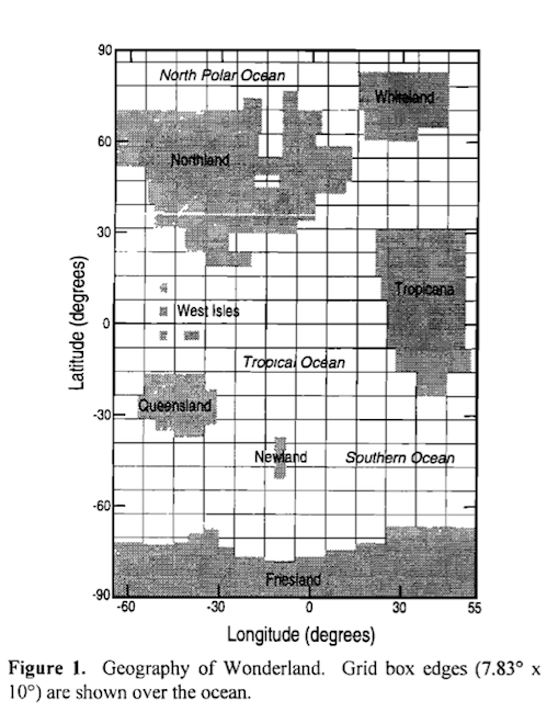
From Hansen et al (1997)
Figure 1
Wonderland is then used in Radiative Forcing and Climate Response, Hansen, Sato & Ruedy (1997). The authors say:
We examine the sensitivity of a climate model to a wide range of radiative forcings, including change of solar irradiance, atmospheric CO2, O3, CFCs, clouds, aerosols, surface albedo, and “ghost” forcing introduced at arbitrary heights, latitudes, longitudes, season, and times of day.
We show that, in general, the climate response, specifically the global mean temperature change, is sensitive to the altitude, latitude, and nature of the forcing; that is, the response to a given forcing can vary by 50% or more depending on the characteristics of the forcing other than its magnitude measured in watts per square meter.
In other words, radiative forcing has its limitations.
Definition of Radiative Forcing
The authors explain a few different approaches to the definition of radiative forcing. If we can understand the difference between these definitions we will have a much clearer view of atmospheric physics. From here, the quotes and figures will be from Radiative Forcing and Climate Response, Hansen, Sato & Ruedy (1997) unless otherwise stated.
Readers who have seen the IPCC 2001 (TAR) definition of radiative forcing may understand the intent behind this 1997 paper. Up until that time different researchers used inconsistent definitions.
The authors say:
The simplest useful definition of radiative forcing is the instantaneous flux change at the tropopause. This is easy to compute because it does not require iterations. This forcing is called “mode A” by WMO [1992]. We refer to this forcing as the “instantaneous forcing”, Fi, using the nomenclature of Hansen et al [1993c]. In a less meaningful alternative, Fi is computed at the top of the atmosphere; we include calculations of this alternative for 2xCO2 and +2% S0 for the sake of comparison.
An improved measure of radiative forcing is obtained by allowing the stratospheric temperature to adjust to the presence of the perturber, to a radiative equilibrium profile, with the tropospheric temperature held fixed. This forcing is called “mode B” by WMO [1992]; we refer to it here as the “adjusted forcing”, Fa [Hansen et al 1993c].
The rationale for using the adjusted forcing is that the relaxation time of the stratosphere is only several months [Manabe & Strickler, 1964], compared to several decades for the troposphere [Hansen et al 1985], and thus the adjusted forcing should be a better measure of the expected climate response for forcings which are present at least several months..The adjusted forcing can be calculated at the top of the atmosphere because the net radiative flux is constant throughout the stratosphere in radiative equilibrium. The calculated Fa depends on where the tropopause level is specified. We specify this level as 100 mbar from the equator to 40° latitude, changing to 189 mbar there, and then increasing linearly to 300 mbar at the poles.
[Emphasis added].
This explanation might seem confusing or abstract so I will try and explain.
Let’s say we have a sudden increase in a particular GHG (see note 1). We can calculate the change in radiative transfer through the atmosphere with a given temperature profile and concentration profile of absorbers with little uncertainty. This means we can see immediately the reduction in outgoing longwave radiation (OLR). And the change in absorption of solar radiation.
Now the question becomes – what happens in the next 1 day, 1 month, 1 year, 10 years, 100 years?
Small changes in net radiation (solar absorbed – OLR) will have an equilibrium effect over many decades at the surface because of the thermal inertia of the oceans (the heat capacity is very high).
The issue that everyone found when they reviewed this problem – the radiative forcing on day 1 was different from the radiative forcing on day 90.
Why?
Because the changes in net absorption above the tropopause (the place where convection stops and let’s review that definition a little later) affect the temperature of the stratosphere very quickly. So the stratosphere quickly adjusts to the new world order and of course this changes the radiative forcing. It’s like (in non-technical terms) the stratosphere responded very quickly and “bounced out” some of the radiative forcing in the first month or two.
So the stratosphere, with little heat capacity, quickly adapts to the radiative changes and moves back into radiative equilibrium. This changes the “radiative forcing” and so if we want to work out the changes over the next 10-100 years there is little point in considering the radiative forcing on day 1, but maybe if the quick responders sort themselves out in 60 days we can wait for the quick responders to settle down and pick the radiative forcing number after 90-120 days.
This is the idea behind the definition.
Let’s look at this in pictures. In the graph below the top line is for doubling CO2 (the line below is for increasing solar by 2%), and the top left is the flux change through the atmosphere for instantaneous and for adjusted. The red line is the “adjusted” value:
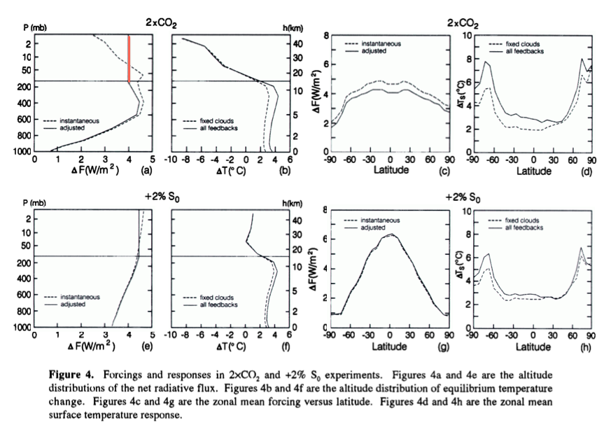
From Radiative Forcing & Climate Response, Hansen et al (1997)
Figure 2 – Click to expand
This red line is the value of flux change after the stratosphere has adjusted to the radiative forcing. Why is the red line vertical?
The reason is simple.
The stratosphere is now in temperature equilibrium because energy in = energy out at all heights. With no convection in the stratosphere this is the same as radiation absorbed = radiation emitted at all heights. Therefore, the net flux change with height must be zero.
If we plotted separately the up and down flux we would find that they have a slope, but the slope of the up and down would be the same. Net absorption of radiation going up balances net emission of radiation going down – more on this in Visualizing Atmospheric Radiation – Part Eleven – Stratospheric Cooling.
Another important point, we can see in the top left graph that the instantaneous net flux at the tropopause (i.e., the net flux on day one) is different from the net flux at the tropopause after adjustment (i.e., after the stratosphere has come into radiative balance).
But once the stratosphere has come into balance we could use the TOA net flux, or the tropopause net flux – it would not matter because both are the same.
Result of Radiative Forcing
Now let’s look at 4 different ways to think about radiative forcing, using the temperature profile as our guide to what is happening:
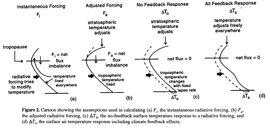
From Radiative Forcing & Climate Response, Hansen et al (1997)
Figure 3 – Click to expand
On the left, case a, instantaneous forcing. This is the result of the change in net radiation absorbed vs height on day one. Temperature doesn’t change instantaneously so it’s nice and simple.
On the next graph, case b, adjusted forcing. This is the temperature change resulting from net radiation absorbed after the stratosphere has come into equilibrium with the new world order, but the troposphere is held fixed. So by definition the tropospheric temperature is identical in case b to case a.
On the next graph, case c, no feedback response of temperature. Now we allow the tropospheric temperature to change until such time as the net flux at the tropopause has gone back to zero. But during this adjustment we have held water vapor, clouds and the lapse rate in the troposphere at the same values as before the radiative forcing.
On the last graph, case d, all feedback response of temperature. Now we let the GCM take over and calculate how water vapor, clouds and the lapse rate respond. And as with case c, we wait until the temperature has increased sufficiently that net tropopause flux has gone back to zero.
What Definition for the Tropopause and Why does it Matter?
We’ve seen that if we use adjusted forcing that the radiative forcing is the same at TOA and at the tropopause. And the adjusted forcing is the IPCC 2001 definition. So why use the forcing at the tropopause? And why does the definition of the tropopause matter?
The first question is easy. We could use the forcing at TOA, it wouldn’t matter so long as we have allowed the stratosphere to come into radiative equilibrium (which takes a few months). As far as I can tell, my opinion, it’s more about the history of how we arrived at this point. If you want to run a climate model to calculate the radiative forcing without stratospheric equilibrium then, on day one, the radiative forcing at the tropopause is usually pretty close to the value calculated after stratospheric equilibrium is reached.
So:
- Calculate the instantaneous forcing at the tropopause and get a value close to the authoritative “radiative forcing” – with the benefit of minimal calculation resources
- Calculate the adjusted forcing at the tropopause or TOA to get the authoritative “radiative forcing”
And lastly, why then does the definition of the tropopause matter?
The reason is simple, but not obvious. We are holding the tropospheric temperature constant, and letting the stratospheric temperature vary. The tropopause is the dividing line. So if we move the dividing line up or down we change the point where the temperatures adjust and so, of course, this affects the “adjusted forcing”. This is explained in some detail in Forster et al (1997) in section 4, p.556 (see reference below).
For reference, three definitions of the tropopause are found in Freckleton et al (1998):
- the level at which the lapse rate falls below 2K/km
- the point at which the lapse rate changes sign, i.e., the temperature minimum
- the top of convection
Conclusion
Understanding what radiative forcing means requires understanding a few basics.
The value of radiative forcing depends upon the somewhat arbitrary definition of the location of the tropopause. Some papers like Freckleton et al (1998) have dived into this subject, to show the dependence of the radiative forcing for doubling CO2 on this definition.
We haven’t covered it in this article, but the Hansen et al (1997) paper showed that radiative forcing is not a perfect guide to how climate responds (even in the idealized world of GCMs). That is, the same radiative forcing applied via different mechanisms can lead to different temperature responses.
Is it a useful parameter? Is the rate of inflation a useful parameter in economics? Usefulness is more a matter of opinion. What is more important at the start is to understand how the parameter is calculated and what it can tell us.
References
Radiative forcing and climate response, Hansen, Sato & Ruedy, Journal of Geophysical Research (1997) – free paper
Wonderland Climate Model, Hansen, Ruedy, Lacis, Russell, Sato, Lerner, Rind & Stone, Journal of Geophysical Research, (1997) – paywall paper
Greenhouse gas radiative forcing: Effect of averaging and inhomogeneities in trace gas distribution, Freckleton et al, QJR Meteorological Society (1998) – paywall paper
On aspects of the concept of radiative forcing, Forster, Freckleton & Shine, Climate Dynamics (1997) – free paper
Notes
Note 1: The idea of an instantaneous increase in a GHG is a thought experiment to make it easier to understand the change in atmospheric radiation. If instead we consider the idea of a 1% change per year, then we have a more difficult problem. (Of course, GCMs can quite happily work with a real-world slow change in GHGs. And they can quite happily work with a sudden change).


sod:
Thanks for raising the discourse level.
This post gets to the crux of forcing.
I have a few comments:
1. If you have time, I have an idea for a posting.
That is: do a radiative calculation for 2xCO2 ( both instantaneous and adjusted ) for a winter sounding over the South Pole. Myhre indicated that three soundings should suffice for a global forcing estimate, and that may be, but I think the South Pole winter sounding merits an investigation. South Pole is 89009 available here: http://weather.uwyo.edu/upperair/sounding.html
June 22 would be a good date.
2. It seems that some of the assumptions ( adjusting the stratosphere first, for example ) amount to a computational concurrency issue ( radiative calculations first, then atmospheric calculations later, in realtiy all processes are continual ).
3. The stratosphere is assumed to be in radiative equilibrium. But there is Stratosphere-Troposphere exchange. And if the stratosphere does cool ( as the change in cooling rates from CO2 increase indicates ) and the troposphere warms, then ST exchange increases the heat transfer.
4. Radiative transfer models indicate a decrease in the net at the top of the troposphere but also indicate an increase in downward radiation at the bottom of the troposphere ( that is into the surface ). How much of this excess bubbles up to the tropopause, thus reducing the imbalance there?
Great topic – keep up the good work.
I find that the concept of radiative forcing only makes sense for instantaneous increases in GHGs. This is because it assumes a radiative imbalance between before and afterwards. So for example an instantaneous doubling of CO2 causes a radiative forcing of ~ 3.6 watts/m2. Within 50 years or so the atmosphere would then settle down to a new energy balance with a slightly modified temperature profile, perhaps with the tropopause slightly higher in altitude. So if the increase takes place very slowly then at each moment in time the climate would be in energy balance and the net forcing is always zero. The current situation on Earth is somewhere between these 2 cases. Man has been increasing CO2 levels for 150 years. The “forcing” from <50 years ago has already worked through the system.
I once looked at this "inertia effect" based on an old version of the GISS GCM model. I fitted a response curve
DT(y) = DT0(1-exp(y/15))
where DT0 is the final response (surface) temperature change and y is the number of years following the increase in forcing. In other words the forcing also decays with an e-folding time of 15 years.
Isaac Held’s posts from March 2011 discuss the issue of, how various time scales enter very well
http://www.gfdl.noaa.gov/blog/isaac-held/2011/03/
The range of relevant time scales is wide. On the shortest side we have the purely radiative effects and reaching the local thermal equilibrium at the modified level of radiation. All that takes much less than one millisecond, if evaporation and condensation is excluded. On the long side reaching a stationary state for the deepest ocean may take millenia. Between these extremes we have many important timescales and even more of those that are not totally negligible.
Calculating radiative forcing as described in the post is sensible and useful, but it has major weaknesses. Radiative transfer calculations can only predict temperature change at locations where energy is transferred only by radiation. Since convection also transfers energy at most places in the troposphere, radiative forcing is of little value in predicting what will happen there. A radiative imbalance at the tropopause caused by a step-function increase GHGs will eventually produce enough warming somewhere below the tropopause to restore the balance – but the radiative forcing alone can’t predict where this warming must occur and therefore how big it must be. The most likely location is the altitudes that already emit most of the photons that escape to space, and most of those come from far above the surface. In theory, a radiative imbalance at the tropopause can be corrected without any surface warming. Thus we are stuck with using GCM’s to predict where and how much warming will occur before a radiative imbalance is corrected.
There may be some merit in considering the “surface radiative forcing”. As we can see from SOD’s Figure 2 (Hansen’s Figure 4), the radiative imbalance at the surface caused by doubling CO2 is calculated to be slightly less than 1 W/m2. (The reduced forcing occurs because water vapor and CO2 absorptions overlap. When the high humidity near the surface is already intercepting most of the photons emitted by the surface, doubling CO2 has little effect.) If we instantly double CO2, DLR will increase by 1 W/m2, from 333 to 334 W/m2 on the KT energy balance diagram. There are several routes by which this 1 W/m2 imbalance can be corrected: 1) The surface can warm by 0.18 degK, or 2) convective energy flux can increase from 97 to 98 W/m2, or 3) some combination of the two can occur. Any warming that occurs can amplified by water vapor and other feedbacks
High in the troposphere, there is much less water vapor to compete with CO2 for intercepting upward photons, so the radiative forcing for 2X CO2 is much larger (3.7 W/m2). If the average photon escaping to space is emitted from GHG’s at 255 degK (the blackbody equivalent temperature), a 1 degC rise is needed to increase outward radiation by 3.7 W/m2. This warming can be amplified by amplified by feedbacks.
Before feedbacks, we have more warming above the surface than at the surface, meaning that the lapse rate will decrease. Since convection is driven by an unstable (high) lapse rate, we might anticipate a decrease in convection rather than an increase. (If we arbitrarily insist the the lapse rate remains constant, the surface must warm as much as the upper atmosphere.) The real problem is that the settled physics of atmospheric radiation can’t predict surface warming and we all know that GCM’s have dubious ability to model convection. Our host can write elegant post after elegant post about radiation, but the real crux of the global warming issue is modeling convection and feedbacks.
Frank,
No-feedback warming is commonly defined as having the same lapse rate. Thus the lapse rate cannot change unless the definition is changed.
As we cannot ever have a no-feedback situation, we are free to define it’s details in various ways.
From the constancy of the lapse rate and radiative changes we can calculate the changes in convection.
Pekka: When I first started teaching myself about climate science, I was frustrated that the effects of GHGs were always reported in terms of W/m2, rather than a temperature change. If one doesn’t get distracted by technical definitions (such as your definition of “no-feedbacks”), there is a very simple method to convert a forcing in terms of W/m2 into a temperature change that is rarely made clear. IMO, climate scientists avoid this simplicity because they don’t want the public to know how small the no-feedbacks climate sensitivity really is – and this is the only part of AGW that might be called “settled science”. If you pick any temperature, it’s easy to calculate how much that temperature must rise so that 3.7 W/m2 (to compensate for 2XCO2) more blackbody radiation is emitted. The mathematically inclined can differentiate the S-B equation and rearrange to the terms to get an equation I found in one of Hansen’s early papers, but don’t see elsewhere. Independent of emissivity, the equation basically says that the percent change in temperature will be 1/4 the percent change in radiation for small changes in radiation:
dW/W = 4*(dT/T)
The question that initially stumped me was: What temperature should I pick? Finally I convinced myself that the blackbody temperature equivalent to the absorbed solar radiation (239 W/m2 == 255 degK) was the most relevant temperature. The average photon passing through the tropopause is emitted from molecules with an average temperature of about 255 degK, which is approximately 5 km above the surface. To emit 3.7 W/m2 more radiation, the average temperature needs to rise 1.0 degC (to 256 degK). The calculated no-feedback climate sensitivity of 1.0 degK is reasonably close to the answer produced by GCMs (1.2 degK), it could be presented in a high school physics course, and has only some minor fudging (the emissivity of the atmosphere isn’t 1 and the fourth root of the average of a range of T^4’s isn’t exactly T).
I object to disrupting the clarity of this reasonably accurate picture (assuming it is reasonably accurate). Most of the photons leaving the earth come from high in the troposphere (about 5 km) and THAT LOCATION – not the surface – will need to warm an average of about 1 degK to compensate for the radiative forcing of 2X CO2. Without the help of a GCM or ARBITRARILY postulating a fixed lapse rate, this simple physics can’t tell us how much the surface will warm. Postulating a fixed lapse rate is a needless complication that appears totally arbitrary! A decrease in the lapse rate from 6.5 to 6.3 degK/km could negate all warming from 2XCO2 at the surface and simple physics doesn’t tell us whether the global average lapse rate should be 6.5 or 6.3 degK/km!
This simple picture can be supplemented with water vapor and other feedbacks. Increased humidity reduces the maximum stable lapse rate (a theoretical figure), but the ENVIRONMENTAL lapse rate is determine by other factors, especially convection.
Frank,
I’m with you in thinking that the the main purpose for introducing the no-feedback climate sensitivity is to express the forcing in the temperature unit which has more intuitive meaning that the forcing expressed as power per unit area. I do also agree that it should be calculated as the change in effective radiative temperature. As you describe we need only the Stefan-Boltzmann law to make that conversion. (I have argued elsewhere for this approach a year or two ago.)
The change in effective radiative temperature would be a real change in a rapid doubling in CO2 concentration, not an artificially defined change as the no-feedback change of the surface temperature. The numbers differ a little (20-30%), but determining, how much they differ is already a rather complex calculation. It would be more straightforward to use directly the change in the effective radiative temperature.
Finally neither one really matters but we wish to know the change including at least the rapid feedbacks. Therefore the no-feedback sensitivity is just an unnecessary complication that adds little to the consideration. Unfortunately it has been used already so much that it’s not possible to get rid of it any more.
Frank,
No, it can’t. We’ve been over this before. You’re neglecting the fact that changing the lapse rate changes the average temperature of the atmosphere. That changes emission. In your example, keeping the surface temperature constant by reducing the lapse rate increases downwelling radiation at the surface causing a radiative imbalance. So changing the lapse rate has much the same effect as changing the CO2 concentration. Now you might argue that convection would increase to make up the difference. But increased convection with a decreased lapse rate is the opposite of what you would expect to happen based on the physics of the atmosphere. The lapse rate is what it is for a reason. The fact that the reason isn’t simple physics is irrelevant.
Frank and DeWitt,
It’s a well known fact that the lapse rate feedback is negative, but as DeWitt explained lapse rate changes only for a reason. That reason is typically increased moisture, but increased moisture means more absorption by water vapor, i.e. a positive water vapor feedback.
Model calculations have shown that the combined effect of the positive water vapor feedback and the negative lapse rate feedback is weakly positive. It has also been stated that different models give consistently similar values for the combined effect even when the vary more for the two components separately. (I have not looked in detail on this issue, but this is, how it has typically been explained.)
Pekka,
Lapse rate feedback is only negative at the TOA. It’s positive at the surface. If you have a radiative imbalance at the TOA, say from doubling CO2, you can get rid of it by decreasing the lapse rate while keeping the surface temperature constant, i.e. warming the upper atmosphere. But the energy imbalance in the system still exists. It’s just been moved to the surface because downwelling radiation has increased by about the same amount it was increased at the TOA while the surface upward emission remains constant.
The same thing happens at the surface if you keep the lapse rate constant and increase the surface temperature because downward atmospheric emission increases faster than upward surface emission. But at higher surface temperature, increased convection to balance the books would be physically realistic.
DeWitt,
Feedback is in general discussed in terms of surface temperatures. A negative feedback is a mechanism where an increase in the surface temperature causes changes in the atmosphere which brings the surface temperature closer to the original value.
The lapse rate feedback works by raising the temperature at high altitudes when the surface temperature is kept fixed. That leads to additional radiation to space and cools the Earth system and the surface as part of that.
Pekka,
Not exactly, IMO. A negative feedback is a mechanism that prevents the surface temperature from increasing as much as it would without the negative feedback. Your statement would imply overshoot and correction. And you’re still ignoring the consequences of increased downward atmospheric radiation at the surface from decreasing the lapse rate. In fact, the result would be to restore the original lapse rate by warming the surface and cooling the upper atmosphere. Which brings me back to what I originally said to Frank: You can’t use the lapse rate alone as a negative feedback to reduce the surface temperature change from, say, doubling CO2. It isn’t an arbitrarily adjustable variable.
Pekka,
An arbitrary lapse rate is also a fundamental problem with radiative/convective models from simple 1D to AOGCM’s. The lapse rate ideally should be an emergent property of the system, not a somewhat arbitrary value defined by the programmer. Note that using the adiabatic lapse rate, moist or dry, is still arbitrary as the environmental lapse rate above the surface boundary layer is almost always less than the adiabatic rate. But that would require actually calculating convection rather than doing a convective energy balance with an arbitrary lapse rate. But that’s not really possible at the moment and it’s not clear that it will ever be possible as it requires solving Navier-Stokes at a quite small minimum dimension, on the order of a centimeter or smaller rather than 100 km.
DeWitt,
Overshoot and correction are dynamical issue, but I haven’t said anything about dynamics.
It’s a normal practice to describe feedbacks as I have done, but without dynamics it’s not really possible to say that we have first one phenomenon and the a correction to that. For a non-dynamical system a negative feedback is always a factor that makes the real effect smaller that it would be without the feedback. This is the sense I have discussed the feedback.
A non-dynamical negative feedback is always weaker than the effect without feedback. It can never reverse the sign of the effect. This is a simple logical conclusion. Dynamical feedbacks may lead to overshoots and oscillations, but that’s a different issue.
Thus your formulation
is fully in agreement with what I meant by my comment.
You should check what “lapse rate feedback means”. I’m pretty sure it means exactly what I wrote. Nothing in your additional comments is relevant for the main point. The Earth energy balance is determined at TOA. Therefore the significant factor is the temperature difference between the surface and upper troposphere at some fixed altitude. This temperature difference is directly dependent on the lapse rate.
I’m not ignoring anything, I’m only keeping the concepts well defined.
I have already agreed that the lapse rate cannot be set arbitrarily, nothing in the physical world can. Everything must be consistent with the other factors. I did also emphasize that the lapse rate feedback and the water vapor feedback change together. Both get stronger with more moisture, and the source for the additional moisture is warmer surface, in particular warmer tropics. The positive water vapor feedback changes more than the negative lapse rate feedback. Therefore the overall feedback excluding cloud feedback is positive.
The local lapse rate must be rather close to the adiabatic one (moist or dry depending of the case) in both ascending and subsiding convection, but vertical convection does not take place everywhere. Therefore the environmental lapse rate is smaller than the dry adiabatic lapse rate even when the relative humidity is well below 100%. As the environmental lapse rate is an effective value in an inhomogeneously behaving atmosphere, where horizontal mixing is also important, its precise value is certainly difficult to calculate from theoretical models.
Whether it would be necessary to go the the level of centimeters in the fluid dynamical calculations is not obvious, but modeling turbulent flows is certainly difficult independently of that.
Pekka,
It depends on what you mean by close and everywhere. Some sort of convective energy transfer must occur everywhere where it is required to sustain energy balance. On average, ignoring temperature inversions at very high latitudes in the winter, that’s pretty much everywhere in the lower atmosphere most of the time. If the atmosphere is stable, i.e. θe is constant with altitude, what is going to drive convection? Constructing a θe vs altitude or log P plot is instructive. I’m in the process of doing one for the standard tropical atmosphere. Assuming I’ve done it correctly, θe decreases from 72C at the surface to 51C at 5km, is about constant to 7 km and increases to 75 C at 12km. That means the lower 5km isn’t stable, which isn’t surprising considering that vertical energy transfer there is significant. I suspect that SoD’s test atmospheres with their sharp drop in humidity above the surface layer are highly unstable too. And an atmosphere with a constant θe with altitude is going to be radiatively unstable.
Momentum is important too. In the strong updrafts in a thunderstorm, for example, a parcel will be carried far above its equilibrium position. IMO, it isn’t possible to understand the atmosphere without considering dynamics.
Pekka,
Here’s the plot for the MODTRAN Tropical Atmosphere. As you can see, it’s adiabatic nowhere. IMO, it’s not even particularly close. For lurkers, if it were adiabatic, it would be a vertical straight line, i.e. constant with altitude.
Just to add my centsworth in response to many of the comments, especially DeWitt Payne’s more recent comment of March 3, 2013 at 2:20 am.
The actual measured lapse rate is not simple to explain.
The Tropics
The annual average of equivalent potential temperature is almost vertical in the tropics:
Click to Expand
For newcomers, this is the same as saying that the temperature profile follows the moist adiabatic lapse rate (at least for the annual average).
On large-scale circulations in convecting atmospheres, Emanuel, Neelin & Bretherton, QJR Meteor. Soc. (1994) is a good paper to explore for this subject. I’m going to try and take my own advice and study it.
Mid-Latitudes and Polar Regions
The lapse rate outside the tropics is not at all easy to explain. The measured lapse rate does not follow the dry adiabatic lapse rate. This is due to the dynamics of the atmosphere in the extra-tropics.
For example, from Stone & Carlson (1979):
Sod,
Your graphs is a good entry to the discussion, where the main problem has probably been the difficulty in communicating through short comments.
When and where vertical convection with little horizontal or turbulent mixing takes place, the lapse rate must be very close to the adiabatic one (dry or moist). That follows directly from thermodynamics and the assumption of little mixing.
That the average lapse rate is not the adiabatic lapse rate for average conditions tells that something more is going on. Your graph tells that the tropical moist updraft is stable and dominant enough to maintain the moist adiabat lapse rate even in the annual average, while the variability makes elsewhere the average lapse rate to differ both from the moist and the dry lapse rate. The environmental lapse rate is not the outcome of any specific local conditions but rather the net result, when many different local conditions combine to maintain some kind of effective average.
I really hate the new format photobucket. Once upon a time, the direct link was only to the image. Now it goes to the whole library. I don’t understand the attraction of the library thing. It’s everywhere now. PowerDVD 12 is particularly bad. If you switch to cinema mode, it forgets your library and has to search the disk all over again when you switch back, which you have to do because you can’t view video clips in cinema mode.
I’ve updated the graph to include the other atmospheres in MODTRAN. Using equivalent potential temperature makes the Sub-Arctic Winter temperature inversion much more obvious.
If you averaged vertical slices of SoD’s plot from -30 to 30 latitude, I suspect it would look a lot like the MODTRAN tropical atmosphere plot. Almost vertical isn’t vertical. θe is still higher at the surface then decreases before increasing again.
It is nice to see that Pekka agrees that convection can happen with an adiabatic lapse rate. He seemed to me to be arguing rather strongly elsewhere that it can’t.
DeWitt,
Evidently I couldn’t present my views clearly enough. Being concise is a virtue in net discussion, but it’s often also problematic as it may lead to misunderstandings. I haven’t changed my views, but restating them in a slightly different context may make them better understood.
Averaging over the range 30S to 30 N leads to significant variability with altitude but in the range from equator to 20N the deviations from moist adiabat are small.
Frank,
Just to clarify the reason for writing the elegant posts – and thanks for the kind words on my creative writing – many people write comments stating how the radiative physics described by climate science is clearly wrong because — insert invalid handwaving argument here.
And so this series, like earlier ones, is my attempt to assist with understanding of the indisputable basics – rather to do a snow job on covering up the difficult bits of climate science.
Frank,
As we will see in the next article on this – and as can be seen by anyone reading the referenced (free) paper by Hansen et al, the GCMs predict that the warming and the forcing are not linked geographically. So it is crystal clear that radiative forcing at location x does not relate to temperature rise at location x.
The whole idea of radiative forcing is that some approximations can be made that might (with the appropriate understanding) be useful – just like the rate of inflation.
But even for radiative forcing, Hansen and his co-authors demonstrate that for the simplified model of Wonderland the temperature response is significantly different even for the same forcing depending on how and where it is applied.
[…] 2013/02/21: TSoD: Wonderland, Radiative Forcing and the Rate of Inflation […]
SoD,
Interesting article. Is it fair to ask what the physical basis is in support of incremental GHG absorption being equal to incremental post albedo solar forcing? Is this addressed anywhere in the literature?
Given the following, this seems dubious to me:
1. GHGs are not an energy source (all they can do is re-direct the energy supplied into the system by the Sun).
2. The energy absorbed by GHGs is subsequently re-radiated both up and down.
3. Post albedo solar forcing is not only an energy source, but all in the acting radiating downward (i.e. all flowing in the direction toward the surface).
4. All the energy that enters the atmosphere, either from the top or bottom, has two potential exits paths out of the atmosphere (either to the surface or out into space).
RW,
Let me rephrase your points to make them more accurate:
1.
GHG’s areThe surface is not an energy source (ignoring the miniscule contribution of geothermal energy from radioactive decay in the Earth’s core) ( alltheyit can do is re-direct the energy supplied into the system by the Sun).2. Most of the energy absorbed by the surface is subsequently lost by convection and radiation to the atmosphere, consequently the GHG’s in the atmosphere
and issubsequentlyre-radiatedboth up and down, but mostly down because the atmosphere is mostly opaque and it’s warmer at the bottom than the top. Some of the energy absorbed by the surface is radiated directly to space.3. [No change, irrelevant]
4. All the energy that
entersis absorbed by the atmosphere, either from the top or bottom, comes from the sun and hastwo potentialone exitpathspath,(either to the surface or out into space)out of the atmosphere to space.Perhaps no. 1 is better phrased:
Energy emitted by GHGs, either directly or by transfer to the atmosphere (and subsequently emitted by the atmosphere), is not an energy source (it is only energy re-directed from that supplied into the system by the Sun).
No. 2 might be better phrased:
The energy absorbed by GHGs is radiated both up and down (i.e. both toward the surface and away from the surface).
No. 3 is totaly relevant, because of nos. 1 & 2 (especially no. 2). That is, post albedo solar power is all flowing in the direction toward the surface (i.e. all acting to warm), where as the power absorbed by GHGs is not.
I stand behind no. 4. Every joule that enters the atmosphere, regardless of how it enters the atmosphere, has the potential to exit the atmosphere over twice the area it arrives from (i.e. either to the surface or out into space).
Or that is, in from the top (Sun) and potentially out the top or bottom, or in from the bottom (surface) and potentially out the top or bottom.
RW,
A really long time ago (1800s) scientists proved the first law of thermodynamics. This says that 1 Joule is 1 Joule and will be conserved regardless of whether it was brought in on a horse and cart or arrived via radiation.
You have some hand-waving argument about how 1 extra Joule from the sun absorbed in the climate system gets dealt with differently from 1 extra Joule that is prevented from leaving the climate system.
I long since lost interest in asking you to write down an equation that justified this hypothesis.
SoD,
“A really long time ago (1800s) scientists proved the first law of thermodynamics. This says that 1 Joule is 1 Joule and will be conserved regardless of whether it was brought in on a horse and cart or arrived via radiation.
Yes, agreed. This is actually the fundamental physical basis behind the contention I’m making.
You have some hand-waving argument about how 1 extra Joule from the sun absorbed in the climate system gets dealt with differently from 1 extra Joule that is prevented from leaving the climate system.
Yes, this is it exactly. Climate science assumes both are equal in their ability to act to ultimately warm the surface, right? That is, it is claimed in the absence of feedback, each would elevate the surface temperature by the same amount, right? This is key distinction, because I certainly agree that on an energy quantitative basis they are equal, as afterall a watt is watt, a joule is a joule, independent of where it last originated from (i.e. can only do the same amount of work).
I long since lost interest in asking you to write down an equation that justified this hypothesis.
I’m not sure this can be demonstrated by an equation, as any equation is only as good as the assumptions and definitions going into it. Being wrong about the physical meaning of incremental GHG absorption has certainly chasened me, but I still don’t think anyone (yourself included) has provided a clear line of evidence and logic in support of the contention that incremental GHG absortpion is equal to incremental post albedo solar forcing (as claimed).
Let me try to explain fundamentally what my objection is and why:
1. Every definition of the GHE, including the one from the IPCC, uses language similar to this one from wikipedia:
The greenhouse effect is a process by which thermal radiation from a planetary surface is absorbed by atmospheric greenhouse gases, and is re-radiated in all directions. Since part of this re-radiation is back towards the surface and the lower atmosphere, it results in an elevation of the average surface temperature above what it would be in the absence of the gases.
That is, the fundamental mechanism is the absorption of upwelling radiation acting to cool that is absorbed and subequently re-radiated back downwards (i.e. radiative resistance to cooling), and specifically not through some sort of conduction process (i.e. the primary way energy is transferred from the atmosphere to the surface is by radiation – not by conduction)
2. Each layer of the atmosphere that absorbs upwelling radiation subsquently radiates that absorbed energy both up and down. I fail to understand how this would somehow not have to be accounted for. Is absorbed radiative energy re-emitted up in the atmosphere not part of the radiative cooling process in the system (i.e. in the act of cooling and not warming)?
To me, if the 3.7 W/m^2 is just a quantification of the reduction in upwelling radiation that was all prior passing out to space and not a quantification of 3.7 W/m^2 in the act of radiating downward (or more specifically back downward), I don’t understand how it can be considered equal to 3.7 W/m^2 of additional post albedo solar power which is all in the act of radiating downward (i.e. a continuous stream of downward radiated energy flowing into the whole Earth-atmosphere system, all in the direction toward the surface).
3. Conservation of Energy. That is, for a state of energy balance, there has to be an equal amount of energy coming out of the atmosphere as is going in, and there are only two ways out (either to the surface or out into space – both of which are about equal in area).
Let me further explain:
If, for a state of energy balance, 240 W/m^2 of post albedo solar power enters the system, 240 W/m^2 of LW infrared exits the system at the TOA, and the surface receives a gross of about 490 W/m^2 at a temperature of 288K, this means that there must be an amount equal to 240 W/m^2 in the atmosphere flowing away from the surface towards space, and there must be an amount equal to 490 W/m^2 in the atmosphere flowing toward the surface – for which each must eventually and continuously find its way out of the atmosphere with 240 W/m^2 going to space and 490 W/m^2 going to the surface, right? Otherwise the system would not be in a state of energy balance (i.e. equilibrium).
Now, what is the global average quantification of the flux absorbed by GHGs and clouds? Is it not about 300 W/m^2? If not, what is it about? If it is, where is this flux going? In the steady-state, all of this energy (i.e. power) has to eventually find its way out of the atmosphere, right?
I should also add here (key point):
Fundamentally, I don’t understand why it intuitively makes sense or seems valid to you to assume or consider incremental GHG absorption to be the same as incremental post albedo solar forcing, given the fundamental mechanism for how GHGs elevate the surface temperature above what it would be in their absence is the absorption of upwelling radiation acting to cool that is absorbed and subsequently re-radiated back downwards.
I mean it would be one thing (in the case of GW’s div2) to question and/or not understand that it’s claimed to be virtually exactly half – given the lapse rate, the large amount of convective flux, the non-linearity of all the effects, etc., but another to somehow think it should be considered exactly equal to additional solar forcing. This is what puzzles me.
Why like anything else in engineering and physics does this claim not require quantification and/or demonstration (i.e. some sort of proof)?
Another thing is what dictates (i.e. ultimately determines) the surface temperature is the flow of energy in (and out) of the surface, right? Given the primary way energy flows into the surface is by downward radiation from the atmosphere (and Sun), this would seem to support the contention that downward radiation is the fundamental mechanism acting to warm the surface, right?
It’s also worthy to note that only post albedo solar power from the Sun truly ‘forces’ the system (in a strict definition sense). What additional GHGs really do is modify the system’s response to the forcing of the Sun, which dictates a different equilibrium (i.e. equilibrium surface temperature).
I want to reply to see how far off my conceptual framework is. Please don’t chuckle very loudly. My reply would be it is in the system waiting to leave, part of the internal energy that drives the climate. The longer the wait the more energy in the system to drive the climate. If a ?photon? enters the ground it will either be radiated back to the atmosphere or directly out through the TOA. Thus any ?photon? leaving the atmosphere to the ground is just taking a longer path out of the sytem.
Morris Walters,
Your question is perhaps indicative of one of the difficulties that many have in thinking about what is going on.
A natural way to think is to many the one where you try to follow what happens to a specific input of energy, a “photon”. In the case of the Earth system it’s impossible to follow that approach in practice. Every *photon” releases it’s energy somewhere and the energy goes at that moment to the heat of that local system. That affects almost immediately some energy flows with the neighboring local systems. It’s not possible to follow every path of influence as there are innumerable such paths.
What has to be done is to separate subsystems that have in some way persistent boundaries and to look at their energy balances as a whole. Any change must be studied by comparing the totality formed by the subsystems before and after the change. In some cases also the dynamic equations of the subsystems must be studied. These dynamic equations tell, how the time derivatives of some quantities are related to the momentary state.
The point is that understanding can be improved only trough defining the details and variables in a way that makes writing equations possible and then writing these equations. At the minimum having the knowledge that allows for writing the equations helps even when they have not been explicitly written out.
The never-ending discussion with RW is an example of what happens, when he does not present his concepts well enough for making writing equations possible and when he does not accept the approaches that the science is offering and others are proposing. He rejects what we have, and cannot propose an alternative that would make constructive discussion possible.
The beauty of sciences like physics is that they provide a well defined framework that allows for studying and discussing the phenomena in a well defined way. That allows both for understanding the present scientific knowledge and for discussing its limits, weaknesses, and potential errors. Trying to provide alternatives to the way the issues are described is a demanding task. It’s taken sometimes by scientists, who may search for new productive views, but what we see in the net discussions is usually only an expression of the gaps in the understanding of the people, who have their own “theories”.
Morris,
Similar to the point Pekka makes, heat transfer problems do not track photons.
The Law of the Conservation of Photons and the Law of the Net Path Length of Photons are two laws you don’t find in heat transfer textbooks.
Radiative energy is transferred by photons and then (in the lower atmosphere) thermalized by collisions between all molecules – but what is conserved is energy, measured in Joules.
Heat transfer problems are in concept quite simple because temperature is what drives heat flow. Let’s take the example of an increase in energy absorbed in a body. If there isn’t a high enough temperature differential to drive sufficient energy out of a body then energy is accumulated. If energy is accumulated then temperature increases. Eventually the temperature differential is high enough to cause a high enough heat flow to stabilize the temperature.
The actual steady state or dynamic solution is calculated by using the first law of thermodynamics (energy conservation) and the equations for heat flow via condution, convection and radiation – all three of which rely on the temperatures at any given locations. The dynamic solution also needs the heat capacity to determine the rate of change of temperature.
SoD, Morris, Rw,
I think part of the confusion is the standard definition of the greenhouse effect based on the back radiation argument. I have some sympathy for RW when he questions the wikipedia description:
I also find this to be a red herring !
A much better description is that outlined by SoD above. It is basically a heat transfer problem from the surface to space. Some wavelengths are opaque to IR photons near the surface. Radiation is then in thermal equilibrium with the surrounding air molecules. Photons travel only short distances before being absorbed. As the air thins out with height so the mean free path for photons in these wavelengths increases. For each wavelength there is an “effective emission height” where the mean free path upwards becomes greater than the top of the atmosphere ( i.e. outer space). Photons then escape and cool the atmosphere. When averaged over all wavelengths the net energy loss by radiation must equal the net energy input from the sun.
The effective emission height for wavelengths in the 15 micron band depend on the amount of CO2 in the atmosphere. If this increases then the effective emission height also increases. The key player in the Earth’s heat transfer is the lapse rate and the wavelength averaged effective emission height . The latter essentially defines the tropopause which is where convection stops. It stops there because radiative heat loss dominates. What will actually happen when CO2 increases is more complex than this because no-one really knows how water vapour and clouds will react. I don’t think the IPCC know either.
Continuing on the same basic line.
The greenhouse effect is basically a phenomenon related to radiative heat transfer and nothing else. It’s simply the phenomenon that some wavelengths are not absorbed much by the atmosphere, while the absorption is strong at other wavelengths. That’s important, because solar SW is transmitted much more than thermal IR. I repeat all that to emphasize that’s the GEH is just this combination of absorptive properties of the atmosphere, nothing more and nothing less.
Based on the radiative calculation alone, the effect would make the surface hotter. This is point, where convection enters. Convection is a very nonlinear effect. When the local lapse rate is less than the adiabatic limit, convection does not occur (unless forced), when the lapse rate exceeds the adiabatic limit, convection gets so strong that the limiting value is restored. Convection is not to the least a reason for GHE, but sets an upper limit on it. It’s, however, important that this limit is rather high.
More greenhouse gases lead to better insulation against radiative heat transfer by making the mean free paths of the photons shorter. When the photons are stopped sooner, they cannot transfer heat as effectively than when their mean free path is longer.
It’s possible to discuss back-radiation and other issues, but nothing of that is needed for understanding the GHE.
How about making porridge ?
Put 2 identical pans of water onto a low heat. In one of them now put some porridge oats. The pure water will boil faster than the porridge because the oats make the water more viscous thereby reducing convective/radiative heat losses. If the pan is tall enough then the bottom surface of the porridge will also be hotter.
We may try to explain the issues in simple terms accessible to anyone. To some extent that’s possible, but that approach is of no value when the listener is unwilling to accept the explanation. Simplistic explanations may work only when they are not questioned. They do not contain any real evidence to support them.
It’s also certain that any simplistic explanation of issues like the properties of the atmosphere or global warming is badly incomplete, and often of little value in trying to learn more.
The words of Einstein (possibly rephrased later) apply here again
How true. Oh well, still I’ll be able to clarify my own knowledge, but I won’t have much to offer in return.
clivebest,
I have some sympathy for RW when he questions the wikipedia description:
Actually – no, I think the wikipedia description is accurate. That’s the whole point. If radiative resistance to cooling is the absorption of upwelling radiation acting to cool that is absorbed and subsequently re-radiated back downward, by definition this would not include the amount absorbed and subsequently re-radiated back up in the same direction it was going pre-absorption (i.e. away from the surface. acting to cool). Given an absorbed photon’s energy always has equal probability of being re-radiated up or down until its energy either passes into space or is received by the surface in some form, I’m saying this should have to be accounted for somehow (in some way), because the energy absorbed and re-radiated by GHGs and the atmosphere is not an energy source to the system like post albedo solar power is.
That should say:
Given an absorbed photon’s energy always has equal probability of being re-radiated up or down until its energy either passes into space or is received by the surface in some form, I’m saying this should have to be accounted for somehow (in some way), because the energy absorbed and re-radiated by GHGs in the atmosphere is not an energy source to the system like post albedo solar power is.
RW,
That’s part of every model. Nobody misses that.
You seem to agree on physical principles that must be taken into account, but mostly fail to see that they have been taken into account.
How is it established or demonstrated that in the absence of feedback, a watt of incremental GHG absorption is equal a watt of incremental post albedo solar power in its ability to elevate the surface temperate above what it would otherwise be?
I think it is a red herring because.
I put on some IR goggles activated for just the CO2 15 micron band, and I ascend upwards slowly in a balloon.
– Near the ground I see a thick bright haze in all directions.
– 1 km above the ground it is dimmer but I now begin to see that it is slightly brighter looking downwards than upwards.
– The higher up I go the less bright it gets and the bigger the difference looking up and down becomes.
– About 11 km up it is pitch black looking upwards, but I still see brightness looking down. I measure the radiation intensity looking downwards and plug it into Planck’s distribution – I measure 220K. I measure the temperature of the air outside and find it is also 220K
The surface is not being “heated” by back radiation, nor is any other layer in the atmosphere being heated by the layers above it. The surface and every layer in the atmosphere is losing heat as fast as possible, maximising entropy. There is a net warming of the atmosphere by the surface through radiation, latent heat and convection. The surface is losing heat slightly slower than it would do without any CO2 in the atmosphere.
I calculate that without any CO2 the Earth’s surface temperature would be ~4C colder.
Boiling water in a pot with, or without, a lid, demonstrates the effect of changing the rate of energy loss. And most cooks will know that, even if they can’t say why. I hadn’t thought of oatmeal. The harder one is a practical demonstration of back radiation. But perhaps this is neither the time nor the place to discuss it.
Perhaps a more simplistic way of seeing what I’m trying to get at is this:
Can we agree that if (hypothetically) all the upwelling radiation absorbed by GHGs was re-radiated back up in the same direction it was going pre-absorption, there wouldn’t be a GHE and an elevation of the surface temperature above what it would otherwise be?
No one is willing to answer this?
I also want to clarify something here. Climate science says that in the absence of feedback, +1.1C at the surface is the required amount to get rid of the -3.7 W/m^2 imbalance at the TOA, and not that +1.1C is an amount that would get rid of the imbalance. This is key distinction also, as I agree that if the surface temperature were raised by 1.1C it would get rid of the imbalance.
[…] « Wonderland, Radiative Forcing and the Rate of Inflation […]
If you believe that planetary surface temperatures are all to do with radiative forcing rather than non-radiative heat transfers, then you are implicitly agreeing with IPCC authors (and Dr Roy Spencer) that a column of air in the troposphere would have been isothermal but for the assumed greenhouse effect. You are believing this because you are believing the 19th century simplification of the Second Law of Thermodynamics which said heat only transfers from hot to cold – a “law” which is indeed true for all radiation, but only strictly true in a horizontal plane for non-radiative heat transfer by conduction.
The Second Law of Thermodynamics in its modern form explains a process in which thermodynamic equilibrium “spontaneously evolves” and that thermodynamic equilibrium will be the state of greatest accessible entropy.
Now, thermodynamic equilibrium is not just about temperature, which is determined by the mean kinetic energy of molecules, and nothing else. Pressure, for example, does not control temperature. Thermodynamic equilibrium is a state in which total accessible energy (including potential energy) is homogeneous, because if it were not homogeneous, then work could be done and so entropy could still increase.
When such a state of thermodynamic equilibrium evolves in a vertical plane in any solid, liquid or gas, molecules at the top of a column will have more gravitational potential energy (PE), and so they must have less kinetic energy (KE), and so a lower temperature, than molecules at the bottom of the column. This state evolves spontaneously as molecules interchange PE and KE in free flight between collisions, and then share the adjusted KE during the next collision.
This postulate was put forward by the brilliant physicist Loschmidt in the 19th century, but has been swept under the carpet by those advocating that radiative forcing is necessary to explain the observed surface temperatures. Radiative forcing could never explain the mean temperature of the Venus surface, or that at the base of the troposphere of Uranus – or that at the surface of Earth.
The gravitationally induced temperature gradient in every planetary troposphere is fully sufficient to explain all planetary surface temperatures. All the weak attempts to disprove it, such as a thought experiment with a wire outside a cylinder of gas, are flawed, simply because they neglect the temperature gradient in the wire itself, or other similar oversights.
The gravity effect is a reality and the dispute is not an acceptable disagreement.
The issue is easy to resolve with a straight forward, correct understanding of the implications of the spontaneous process described in statements of the Second Law of Thermodynamics.
Hence radiative forcing is not what causes the warming, and so carbon dioxide has nothing to do with what is just natural climate change.
This comment demonstrates a lack of understanding of what basic atmospheric physics teaches.
Everyone in the field of atmospheric physics (including Dr Roy Spencer) understands that the effect of reducing pressure with height, via the first law of thermodynamics, causes a reduction in temperature.
Potential temperature stays constant.
Actual temperature decreases.
This is all explained in Potential Temperature and Temperature Profile in the Atmosphere – The Lapse Rate. And also in any introductory text in atmospheric physics.
The effect of radiative transfer is on the boundary condition.
Is the outgoing radiation from the surface of the earth in equilibrium with absorbed radiation from the sun?
Or, is the outgoing radiation from the climate system in equilibrium with absorbed radiation from the sun?
SoD,
I agree that the standard texts are all right, but few of them do really discuss the point raised by Climate_Science_Reearcher. I have got involved in related discussions before, and a subthread on this point starts on my site from this comment
It seems really difficult for many people to grasp the true meaning of equipartition theorem and other fundamental laws of physics that explain why Loschmidt was the one who was wrong in his dispute with Boltzmann and others.
Pekka,
I noticed you used a nitrogen atmosphere in one of your comments. No molecular gas will be perfectly transparent in the thermal IR because of collision induced absorption. Sure it’s small, but I’m pretty sure it will easily overwhelm conduction. I’m not sure that even the noble gases qualify either. You need unobtaneon, an ideal gas with properties that are whatever you say they are. It’s similar to the metal unobtanium in that regard.
The whole idea of these counter factual examples is to introduce idealized assumptions, and study their consequences. Real nitrogen may differ from that, but that’s not the point as 100% pure nitrogen atmosphere is as impossible in real universe as an atmosphere of so little absorption that it can be correctly be taken as zero.
One can always argue on the right way of presenting idealized assumptions, and on the value of counter factual examples.
Pekka,
Then why say nitrogen at all? It confuses the issue, IMO.
DeWitt,
The comments on my site are continuation to discussion at Climate etc. I believe that nitrogen was mentioned there, and I believe also that it was agreed that nitrogen was used as code word for a gas totally transparent to IR.
The main sources of IR emissivity of nitrogen must be the N-15 isotope (0.3% of nitrogen) and excited states due to cosmic radiation. Collisions of normal N2 molecules cannot have much effect as the conservation laws restrict their influence as well. The lowest energy line of IR absorption for the mixed isotope N2 is around 3.5 µm. The short wavelength is one additional reason for the near perfect transparency of pure N2 for thermal IR.
The previous comment, full of fairly dubious assertions, is believed to be a sock puppet of one Douglas Cotton, famed climate science crank. He is leaving his droppings at quite a number of websites today
It seems that David Hodge is correct.
The commenter ‘Climate_Science_Reearcher’ appears to be the well-known commenter who was banned from this site for repetition above and beyond any acceptable level and attributing invented claims to others. From time to time he pops up and posts under new identities with new IP addresses.
This blog owes no obligation to invest all of its time on specific individuals just because they are the loudest voices. The readers likewise prefer this policy.
My advice to the same determined individual, as before – start your own blog and write your own stuff and spare us from your amazing insights.
Thanks.
Yes, apparently Doug has access to many IP addresses and can’t even accept being banned (or resist the temptation). Even Roy Spencer has now banned him from his site.
He’s been banned at The Blackboard as well.
Why does it surprise anyone that the radiative forcing models are wrong, when they are not based on valid physics?
[..deleted rest of comment from this banned commenter]
Here we have again one of these comments that claim that climate science is not based on valid physics, but which tells only that the author has no idea of what valid physics is.
The comment is so totally wrong and generic that it’s not possible even to start to correct the errors. The only recommendation I can give is that the author makes some serious effort to learn physics, thermodynamics in particular. Having learned the basics he could come back to this site and extend his knowledge to the more specific issues discussed here.
From the points the basic requirement (1) is the only correct one and that’s, of course, the basis of all application of thermodynamics for atmospheric studies.
Pekka,
It was another comment from someone who has already posted a large number of repetitious comments that are maintained on this blog, and who has posted a large number of the exact same comments that have been deleted.
Not much more to say.
[…] Radiative forcing (for explanation of this term, see for example Wonderland, Radiative Forcing and the Rate of Inflation): […]
[…] In Impacts – II – GHG Emissions Projections: SRES and RCP we looked at projections of emissions under various scenarios with the resulting CO2 (and other GHG) concentrations and resulting radiative forcing. […]
According to AR5 WG1 Section 8.3, the decrease in stratospheric ozone has produced a -0.13 W/m2 LWR radiative forcing (Table 8.3) and the increase in stratospheric water vapor has produced a +0.07 W/m2 forcing. Since the temperature rises with altitude in the stratosphere (albeit weakly around 20 km/50-100 mb in the lower stratosphere), there should be a positive instantaneous forcing (F_i) associated with a decrease in ozone and a negative forcing associated with an increase in stratospheric water vapor. (The opposite of what I expected.) As the stratosphere temperature adjusts and radiative equilibrium is restored, the [adjusted] forcing (F_a) should become zero. If you define forcing as the change at the tropopause (F_2x?), there should be no forcing from any changes in the stratosphere. Table 8.6 makes it clear these values are not ERF’s.
Click to access WG1AR5_SPM_FINAL.pdf
(For what it is worth, the online version of Modtran says that a 10X increase in stratospheric ozone causes no change in OLR at 70 km, suggesting that this calculation has stratospheric adjustment.)
Does anyone understand these counterintuitive results?
Frank,
A large increase in ozone in the stratosphere would result in a large change in stratospheric temperature. Since energy transfer in the stratosphere is essentially radiation only and the heat capacity is low, the temperature would change rapidly. While ozone does absorb and emit in the IR, it’s main effect is by increased absorption of incoming solar radiation. IIRC, Modtran doesn’t allow changes in temperature above about 15km and doesn’t automatically adjust temperatures for changes in atmospheric composition.
Because the temperature increases with altitude in the stratosphere, the greenhouse effect changes sign. IR absorbing/emitting gases which don’t significantly absorb solar radiation cause a decrease in temperature rather than an increase. But I don’t think Modtran, as implemented by Archer on the web, is really able to deal with that.
Overall, addition of water vapor cools the stratosphere while an increase in ozone heats it. The effect of stratosphere temperature change on the surface is more complicated.
DeWitt: Thanks for taking the time to reply. I think we agree upon how ozone and water vapor effect the temperature of the stratosphere, but my question was about the radiative forcing (change in net flux at the TOA) produced by increases in IR-absorbing gases when they are in the stratosphere. There we need to consider the difference between instantaneous radiative forcing (F_i), radiative forcing after the temperature of the stratosphere adjusts to the change in radiative fluxes (F_a), radiative forcing at the tropopause (F_2x, which in theory is approximately the same as F_a).
Click to access 20140011862.pdf
Atmospheric Chemistry and Climate Model Intercomparison Project (ACCMIP)
“By changing the ozone field, heating rates in the stratosphere will have changed. If such a change were to happen in the real atmosphere, stratospheric temperatures would respond quickly (days to months, e.g., Hansen et al., 1997) – much more quickly than the surface-troposphere system, which will adjust on multiannual timescales. A better estimate of the long-term forcing on the surface climate takes into account this short-term response of stratospheric temperatures (Forster et al., 2007). Stratospheric temperature adjustment was achieved by first calculating stratospheric heat- ing rates for the base atmosphere. The stratosphere was asumed to be in thermal equilibrium, i.e. with dynamical heating exactly balancing the radiative heating. Furthermore, the dynamics were assumed to remain constant following a perturbation to ozone. Hence to maintain equilibrium, radiative heating rates must also remain unchanged. To achieve this, stratospheric temperatures were iteratively adjusted in the perturbed case, until stratospheric radiative heating rates returned to their base values. This procedure is called the fixed dynamical heating approximation (Ramanathan and Dickinson, 1979).”
If radiative transfer calculations show non-zero heating (and cooling?) rates at some location, I think this means is that the stratosphere is not in perfect radiative equilibrium. That implies some heat transfer by convection – though not by the buoyancy-driven convection that dominates most of the troposphere. There is the Brewer-Dobson circulation. Apparently, the adjusted forcing associated with a change in the stratosphere need not be zero.
The subject came up in connection with volcanic aerosols and volcanic forcing. Is scattering/reflection the only mechanism by which they interact with radiation? No. These aerosols also warm the stratosphere, so they must absorb SWR, OLR or both. In this respect, these aerosols behave like ozone. We quantify stratospheric aerosols by AOD at 550 nm – extinction (absorption plus scattering) – but that is only a tiny fraction of the information needed to determine calculate forcing.