In Wonderland, Radiative Forcing and the Rate of Inflation we looked at the definition of radiative forcing and a few concepts around it:
- why the instantaneous forcing is different from the adjusted forcing
- what adjusted forcing is and why it’s a more useful concept
- why the definition of the tropopause affects the value
- GCM results usually don’t use radiative forcing as an input
In this article we will look at some results using the Wonderland model.
Remember the Wonderland model is not the earth. But the same is also true of “real” GCMs with geographical boundaries that match the earth as we know it. They are not the earth either. All models have limitations. This is easy to understand in principle. It is challenging to understand in the specifics of where the limitations are, even for specialists – and especially for non-specialists.
What the Wonderland model provides is a coarse geography with earth-like layout of land and ocean, plus of course, physics that follows the basic equations. And using this model we can get a sense of how radiative forcing is related to temperature changes when the same value of radiative forcing is applied via different mechanisms.
In the 1997 paper I think that Hansen, Sato & Ruedy did a decent job of explaining the limitations of radiative forcing, at least as far as the Wonderland climate model is able to assist us with that understanding. Remember as well that, in general, results we see from GCMs do not use radiative forcing. Instead they calculate from first principles – or parameterized first principles.
Doubling CO2
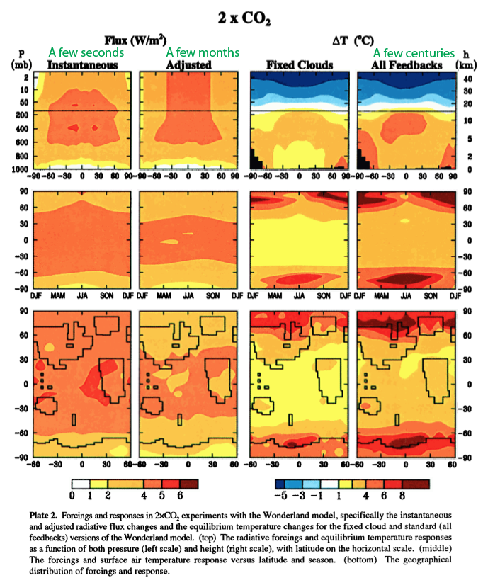
Now there’s a lot in this first figure, it can be a bit overwhelming. We’ll take it one step at a time. We double CO2 overnight – in Wonderland – and we see various results. The left half of the figure is all about flux while the right half is all about temperature:
From Hansen et al 1997
Figure 1 – Green text added – Click to Expand
On the top line, the first two graphs are the net flux change, as a function of height and latitude. First left – instantaneous; second left – adjusted. These two cases were explained in the last article.
The second left is effectively the “radiative forcing”, and we can see that the above the tropopause (at about 200 mbar) the net flux change with height is constant. This is because the stratosphere has come into radiative balance. Refer to the last article for more explanation. On the right hand side, with all feedbacks from this one change in Wonderland, we can see the famous predicted “tropospheric hot spot” and the cooling of the stratosphere.
We see in the bottom two rows on the right the expected temperature change :
- second row – change in temperature as a function of latitude and season (where temperature is averaged across all longitudes)
- third row – change in temperature as a function of latitude and longitude (averaged annually)
It’s interesting to see the larger temperature increases predicted near the poles. I’m not sure I really understand the mechanisms driving that. Note that the radiative forcing is generally higher in the tropics and lower at the poles, yet the temperature change is the other way round.
Increasing Solar Radiation by 2%
Now let’s take a look at a comparison exercise, increasing solar radiation by 2%.
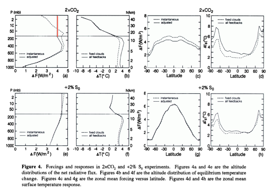
The responses to these comparable global forcings, 2xCO2 & +2% S0, are similar in a gross sense, as found by previous investigators. However, as we show in the sections below, the similarity of the responses is partly accidental, a cancellation of two contrary effects. We show in section 5 that the climate model (and presumably the real world) is much more sensitive to a forcing at high latitudes than to a forcing at low latitudes; this tends to cause a greater response for 2xCO2 (compare figures 4c & 4g); but the forcing is also more sensitive to a forcing that acts at the surface and lower troposphere than to a forcing which acts higher in the troposphere; this favors the solar forcing (compare figures 4a & 4e), partially offsetting the latitudinal sensitivity.
We saw figure 4 in the previous article, repeated again here for reference:
From Hansen et al (1997)
Figure 2
In case the above comment is not clear, absorbed solar radiation is more concentrated in the tropics and a minimum at the poles, whereas CO2 is evenly distributed (a “well-mixed greenhouse gas”). So a similar average radiative change will cause a more tropical effect for solar but a more even effect for CO2.
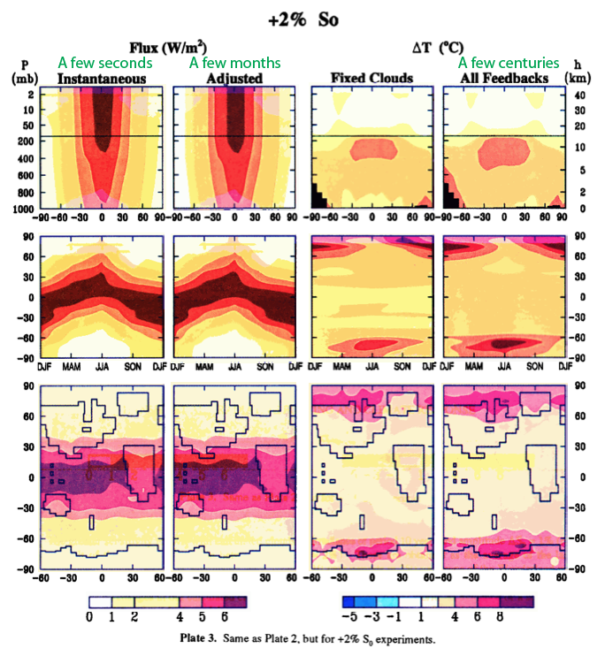
We can see that clearly in the comparable graphic for a solar increase of 2%:
From Hansen et al (1997)
Figure 3 – Green text added – Click to Expand
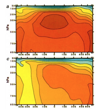
We see that the change in net flux is higher at the surface than the 2xCO2 case, and is much more concentrated in the tropics.
We also see the predicted tropospheric hot spot looking pretty similar to the 2xCO2 tropospheric hot spot (see note 1).
But unlike the cooler stratosphere of the 2xCO2 case, we see an unchanging stratosphere for this increase in solar irradiation.
These same points can also be seen in figure 2 above (figure 4 from Hansen et al).
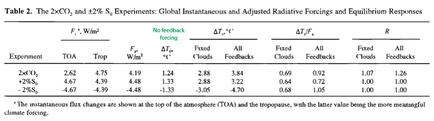
Here is the table which compares radiative forcing (instantaneous and adjusted), no feedback temperature change, and full-GCM calculated temperature change for doubling CO2, increasing solar by 2% and reducing solar by 2%:
From Hansen et al 1997
Figure 4 – Green text added – Click to Expand
The value R (far right of table) is the ratio of the predicted temperature change from a given forcing divided by the predicted temperature change from the 2% increase in solar radiation.
Now the paper also includes some ozone changes which are pretty interesting, but won’t be discussed here (unless we have questions from people who have read the paper of course).
“Ghost” Forcings
The authors then go on to consider what they call ghost forcings:
How does the climate response depend on the time and place at which a forcing is applied? The forcings considered above all have complex spatial and temporal variations. For example, the change of solar irradiance varies with time of day, season, latitude, and even longitude because of zonal variations in ground albedo and cloud cover. We would like a simpler test forcing.
We define a “ghost” forcing as an arbitrary heating added to the radiative source term in the energy equation.. The forcing, in effect, appears magically from outer space at an atmospheric level, latitude range, season and time of day. Usually we choose a ghost forcing with a global and annual mean of 4 W/m², making it comparable to the 2xCO2 and +2% S0 experiments.
In the following table we see the results of various experiments:

Hansen et al (1997)
Figure 5 – Click to Expand
We note that the feedback factor for the ghost forcing varies with the altitude of the forcing by about a factor of two. We also note that a substantial surface temperature response is obtained even when the forcing is located entirely within the stratosphere. Analysis of these results requires that we first quantify the effect of cloud changes. However, the results can be understood qualitatively as follows.
Consider ΔTs in the case of fixed clouds. As the forcing is added to successively higher layers, there are two principal competing effects. First, as the heating moves higher, a larger fraction of the energy is radiated directly to space without warming the surface, causing ΔTs to decline as the altitude of the forcing increases. However, second, warming of a given level allows more water vapor to exist there, and at the higher levels water vapor is a particularly effective greenhouse gas. The net result is that ΔTs tends to decline with the altitude of the forcing, but it has a relative maximum near the tropopause.
When clouds are free to change the surface temperature change depends even more on the altitude of the forcing (figure 8). The principal mechanism is that heating of a given layer tends to decrease large-scale cloud cover within that layer. The dominant effect of decreased low-level clouds is a reduced planetary albedo, thus a warming, while the dominant effect of decreased high clouds is a reduced greenhouse effect, thus a cooling. However, the cloud cover, the cloud cover changes and the surface temperature sensitivity to changes may depend on characteristics of the forcing other than altitude, e.g. latitude, so quantitive evaluation requires detailed examination of the cloud changes (section 6).
Conclusion
Radiative forcing is a useful concept which gives a headline idea about the imbalance in climate equilibrium caused by something like a change in “greenhouse” gas concentration.
GCM calculations of temperature change over a few centuries do vary significantly with the exact nature of the forcing – primarily its vertical and geographical distribution. This means that a calculated radiative forcing of, say, 1 W/m² from two different mechanisms (e.g. ozone and CFCs) would (according to GCMs) not necessarily produce the same surface temperature change.
References
Radiative forcing and climate response, Hansen, Sato & Ruedy, Journal of Geophysical Research (1997) – free paper
Notes
Note 1: The reason for the predicted hot spot is more water vapor causes a lower lapse rate – which increases the temperature higher up in the troposphere relative to the surface. This change is concentrated in the tropics because the tropics are hotter and, therefore, have much more water vapor. The dry polar regions cannot get a lapse rate change from more water vapor because the effect is so small.
Any increase in surface temperature is predicted to cause this same change.
With limited research on my part, the idealized picture of the hotspot as shown above is not actually the real model results. The top graph is the “just CO2” graph, and the bottom graph is the “CO2 + aerosols” – the second graph is obviously closer to the real case:
From Santer et al 1996
Many people have asked for my comment on the hot spot, but apart from putting forward an opinion I haven’t spent enough time researching this topic to understand it. From time to time I do dig in, but it seems that there are about 20 papers that need to be read to say something useful on the topic. Unfortunately many of them are heavy in stats and my interest wanes.


A comment on the warming at high latitudes.
It’s not surprising that the change in subarctic or arctic winter temperature is larger than warming in general. The subarctic winter temperatures change very easily as they are to a significant degree influenced by temperature inversion where radiation through a cold and dry atmosphere is the most important factor. How easily the temperatures vary is seen from the historical variability.
The monthly average temperature for January in Helsinki (60 degrees N) since 1900 has varied between -16.5C and +1.4C. 17.9C is a lot for the variability of monthly average temperature. In Northern Finland around 67N the typical variability is still significantly stronger although the extremes differ only little more (by 19.4C from -24.4C to -5.0C in Sodankylä).
Some graphics on this variability can be seen on the Finnish language page
http://ilmatieteenlaitos.fi/tammikuu
near the bottom of the page.
The variability is much less for July (Heinäkuu in Finnish) (8.0C from 13.7C to 21.7C in Helsinki and 7.5C from 11.0C to 18.5C in Sodankylä).
The large variability of the subarctic surface temperature in winter is an example on, how the surface temperature is not always a good indicator of persistent or slowly changing climatic conditions.
[…] 2013/03/03: TSoD: Wonderland and Radiative Forcing – Part Two […]
The hotspot is more like the ‘not’ spot:
The likely culprit is not radiative but poor capture of the actual physics of convection by the parameterizations.
I believe this means more energy is being lost to the stratosphere than is being modeled.
This doesn’t negate ‘global warming’ but probably lessens the total forcing that we’re currently assuming.
Without the “hot spot” we would miss the negative lapse rate feedback. That should make warming stronger, not weaker.
I hear what you’re saying – the hot spot radiates more effectively because it’s hot.
But what I’m saying is that it doesn’t need to radiate more effectively to approach equilibrium because non-radiative forcing (STE) lessens the actual forcing imposed.
Climate Weenie,
What is “non-radiative forcing”? The forcing is a statement about the energy balance of the Earth, and radiation is the only energy carrier that can contribute to that.
You might mean that the forcing calculated at the tropopause differs more from the forcing at TOA than generally thought. That would require a different net value for the radiative balance of stratosphere with the space, but there are independent limits on the strength of that imbalance. Such limits can be determined from the knowledge on the temperature and chemical profiles of the stratosphere. Satellite observations tell also about that balance.
There are uncertainties in the understanding of the stratosphere, but it’s essential to remember that the stratosphere cannot take more energy from the troposphere than it can transmit to the space (or to the atmosphere above the stratosphere, but this factor is even more restricted).
Why do you think the hot spot has not appeared?
The empirical situation is still not clear. Thus we don’t really know how far the hot spot is there. If the temperature profile does, indeed, differ from what virtually all models predict, the reason would probably be in modeling of the local variability in the atmospheric conditions, i.e., the averages would not follow the idealized case as closely as the parameterizations used in the models imply.
The absence of a THS is a fatal flaw for AGW theory; relevant papers and discussion here:
http://joannenova.com.au/2012/05/models-get-the-core-assumptions-wrong-the-hot-spot-is-missing/
There’s no AGW theory, there’s only theory of the atmosphere. This theory has a lot of successes, but it’s incomplete and fails to describe many details. That theory predicts the influence of CO2 on temperature, but that’s only one of innumerable predictions of the theory.
The idea of a hot spot is based on the dependence of the adiabatic lapse rate on the moisture. The moist lapse rate is smaller than the dry lapse rate and it’s the smaller the higher the absolute moisture level. This means that the moist lapse rate is the smaller the higher the temperature, because the moist lapse rate refers always to state of saturation and the saturation moisture is determined by the temperature.
We can see the absence of the hot spot phenomenon even when we don’t consider any warming, just the present atmosphere. The absence is manifested in the observation that the real average lapse rate is surprisingly constant over a wide range of conditions that differ in temperature and moisture. An average “environmental lapse rate” of about 6.5 C/km has been observed both in tropics and elsewhere. The average rate is not much lower in tropics or higher in dryer areas.
SoD has discussed the lapse rate in several post and shown graphics that tell on some deviations of what I write above, but it remains true that the environmental lapse rate of 6.5 C/km is valid more widely that we might expect from theory. The book Wallace & Hobbs: Atmospheric Science (2nd ed. p. 421) has the comment
By that they tell that the value is not against fundamental principles, but I read there also that this state of matter cannot really be predicted, only found possible. The situation seems to be that the models do tend to predict a lower lapse rate for tropics, and that this effect is in the models getting stronger with warming. The resolution is very likely that the models cannot fully describe the large-scale motions of the above quote. Such a failure would mean that they are not either capable in describing the atmosphere well enough for the calculation of all feedbacks, Most specifically they seem to predict a stronger negative lapse rate feedback than observations support. As water vapor feedback and lapse rate feedback are anticorrelated in models, the error is likely smaller in the sum of these two feedbacks.
If the absence of the hot spot is really confirmed by future research, that tells about a specific weakness of the present models in an area that’s known to be problematic. That’s not to the least influential on other much more strongly justified conclusions of the theory of the atmosphere. Basics of AGW belong to these strongly justified and well understood conclusions. Feedbacks are covered by the more problematic parts of the theory, and to fair extent on the same parts that determine the presence and strength of the hot spot.
Pekka: So there are really two different concerns with the “hotspot” in the upper tropical troposphere. The more publicized problem is that the upper tropical troposphere doesn’t appear to be warming faster than the surface, as predicted by all models. As I understand it, the older radiosonde data has been “homogenized” until the discrepancy disappeared, but satellite data now appear to confirm the discrepancy.
It is very difficult to trust the small difference between surface warming and upper troposphere warming over a period of many decades, so I interested in your comments suggesting a version of the hotspot problem: climate models predict a lower lapse rate (less temperature decrease with altitude) in the tropics than is actually observed. If the upper tropical troposphere is too hot, then convection from the surface will be too low and the surface should be too hot. (Compensating errors might give the right tropical surface temperature.) Is it generally accepted that the tropical lapse rates in models are significantly lower than observed, but that this problem doesn’t occur elsewhere?
Frank,
The value of the actual lapse rate is influenced strongly by horizontal mixing, without horizontal mixing the lapse rate would be always close to either dry or moist lapse rate, but it is not that close. Averaging over time is part of the explanation for a lapse rate that’s between the two adiabatic values, but only a part.
There’s horizontal mixing on many different scales. On local scale air is not rising uniformly but there are commonly both rising and subsiding areas like the thermal columns under cumulus clouds. Turbulent eddies of equally variable sizes are created by these flows and horizontal mixing induced at all altitudes. Calculating from first principles the flows is virtually impossible as calculating turbulent flows is extremely difficult in much simpler cases as well. A lot is known about the atmospheric flows, but modeling them is always inaccurate and involves semiempirical parametrizations. Little can truly be predicted when the questions asked are extrapolations from earlier knowledge rather than interpolation within the empirically studied range.
How the horizontal mixing changes as a consequence of further warming is an example of such extrapolation. Therefore a modest failure in modeling that is not really a serious problem for the trust in the general understanding of the atmosphere, it only tells that the failing models are a little worse than hoped for. Those results that can be derived more directly from basic principles can be considered as certain as before, only phenomena directly influenced by similar details of the model as the rate of warming of the upper tropical troposphere should be considered more uncertain that thought previously.
I tried to write my comment staying within the limits of my knowledge and understanding as a physicist who has only recently learned about atmosphere. A real expert may disagree on some points, and certainly add to what I wrote.
> It’s interesting to see the larger temperature increases predicted near the poles. I’m not sure I really understand the mechanisms driving that.
There is also V A Alexeev et al, Climate Dynamics (2005) 24: 655-666. Which I blogged ages ago at http://mustelid.blogspot.co.uk/2005/07/harry-potter-and-polar-amplification.html
If you believe them, that provides a dynamical-type explanation for polar amplification that is geography-independent.
The emissivity of the stratosphere ( and above ) increases with the addition of CO2.
The stratosphere is modeled to cool with increased CO2 from two factors.
1. It would receive less energy ( radiatively ) from a more opaque troposphere.
2. It would emit more energy ( than a stratosphere with only 1x CO2 )
Part of 1. is lessened if not all of STE is represented by the GCMs
Arctic winter variation is illustrated here. By clicking on the year numbers at the left you can compare earlier and recent years. variation has been impressive all along, but the average temperature has gone up. How much has it increased, by your eye? 4 degrees C?
depends on which year you select as your start point. Eyeballing just seems to reveal lots of variation from year to year
Here is the link:
http://ocean.dmi.dk/arctic/meant80n.uk.php
To the hot spot discussion. I have difficulty in understanding that warming of the upper troposphere is associated with global warming. If climate models come up with a hot spot, a significant increase of warming with increased CO2, at altitudes from 5km to 15 km, then the IR radiation should incrase at those levels. Why would not this result in more radiation to space?
“Therefore, the emission of radiation moves upwards, and “moving upwards” means from a colder part of the atmosphere. Colder atmospheres radiate less brightly and so the TOA flux is reduced. This reduces the cooling to space and so warms the top of the troposphere.” SoD
Is there a contradiction here? Could it continue with: Then it warms the top of the troposphere and so increases cooling to space.
I think you’re missing the point of the flux graphs. The flux is the radiative forcing, so an increase actually means a either a decrease of outgoing flux to space, an increase in downward flux or some combination of both. Note that there is no graph for flux after several centuries. That’s because it would be all white as the forcing would be gone.
The tropospheric hot spot increases emission at the latitudes where it occurs, but the net flux to space from the planet several centuries after doubling CO2 is about the same as it was before the doubling. Note the cooling of the upper troposphere and lower stratosphere at high latitudes. For an increase of 2% of incoming solar radiation, the flux to space from the planet must also increase by 2%.
That being said, it may well be that the hot spot is an artifact of the models and doesn’t happen in the real world.
nobodyknows:
Good question. It would, you are correct.
Warming the surface of the planet causes more radiation to space (through the “atmospheric window” and generally some proportion of surface radiation escapes to space at many wavelengths).
Warming the atmosphere causes more radiation to space – and of course, the more it warms the greater the radiation.
This is a feedback – and it is a negative feedback. It reduces the warming caused by more GHGs, or caused by more solar radiation (or caused by anything).
(It is sometimes called the “Planck feedback”, only by convention. Sometimes the “lapse rate feedback”, but there isn’t a standard term so it depends on the paper in question).
Here is a breakdown of feedbacks from one paper:
It is important to distinguish between what happens as a result of a “forcing” – like more GHGs or more incident solar radiation, and what happens as a result of feedback after that forcing.
So the explanation you cited from me is the initial result of the forcing.
The question you asked “Why would not this result in more radiation to space?” is about the feedback after some warming takes place.
The example is often given of instantaneously doubling CO2. Why this example, since it can’t be instantaneous and takes decades or centuries?
It just helps with conceptual understanding of what takes place due to more CO2 and what takes place as feedbacks after that change.
Hopefully this makes sense. If not, feel free to ask.
nobodyknows,
A decrease in flux to space means an increase in GHG absorption or an increase in atmospheric IR opacity, whether locally in the tropics or globally.
The way the GHE is driven, as I understand it, is by radiative resistance to outer space cooling by radiation from the atmosphere into space. That is, the atmosphere above all must be making the push toward radiative balance at the TOA via IR emitted up toward space, but in order to make that push, it has to push back the other way towards the surface, because absorbed IR is re-radiated by the atmosphere both up and down. The ultimate effect this has (or least theoretically has) is for the lower atmosphere and ultimately the surface to be warmer in order to be pushing through the required IR flux that needs to be passing out the TOA in order to maintain radiative balance with the Sun.
Thank you for the answers DeWitt Payne, Sod and RW. It made it a little more clear to me. I think the different feedbacks are most interesting, and that the lapse rate feedback come out negative. As I understand, the feedbacks from clouds and water vapor are discussed, with less sure magnitudes. So there are some uncertainties. I find the idea that feedbacks are temperature dependent interesting (that sea surface temperatures have more impacts on clouds and latent heat than models show).
I have not seen any descriptions of feedbacks from sun radiation. Should not climate variations (as MWP an LIA) show some amplifications of sun radiation? Could the variations in uv radiation have some impact on climate?
nobodyknows,
The feedback from changing solar radiation has often been a subject of study – as in the paper we looked at in this article: Radiative forcing and climate response, Hansen, Sato & Ruedy.
In very broad terms, a change in radiation of 1W/m2 is a change in 1W/m2 regardless of whether it comes from increased GHGs or increased solar radiation.
This paper demonstrates that looking a little closer (i.e., in less broad terms) we can see that the climate response is not the same.
But back to broad terms, the change in solar radiation needs to be a lot more than we currently see to cause anything like the change from GHGs (see note 1).
In chapter 9 of AR5 (IPCC report) there is a bit of an analysis of the last 1000 years – see 9.5.3 Interannual-to-Centennial Variability.
In that section, models use the forcing reconstructions from Climate forcing reconstructions for use in PMIP simulations of the Last Millennium (v1.1), Schmidt et al (2012).
But the problem with solar radiation is the estimates of past changes rely on ideas (models) that are very difficult to verify. Here is an extract from Schmidt et al:
I don’t know the answer to that one. More detail is probably needed to ask the question – like the details of the change (graph of radiance vs wavelength) and of course it might be interesting to know why it is believed to have occurred.
Note 1: I usually say “all other things being equal” – that is, the calculation of how radiation is absorbed and emitted by the atmosphere as GHGs or solar radiation changes is a simple task (technically demanding but not subject to particular uncertainty). How the climate responds to the changes caused by GHG or solar is of course a trillion times more difficult to work out. Or maybe it is a trillion trillion..
nobodyknows,
“I find the idea that feedbacks are temperature dependent interesting (that sea surface temperatures have more impacts on clouds and latent heat than models show).”
Feedbacks are by definition a response to temperature change, where as some kind of forcing is by definition what causes a temperature change.
The fundamental feedback question rests almost entirely on the what the net combined feedback of clouds and water vapor actually is on global average. Warmer temperatures increase evaporation, which acts to cool the surface cooling, but also increases atmospheric IR opacity via increased water vapor, which by itself acts to further warm the surface. But water vapor acts in tandem with clouds, which have a strong surface cooling effect via their ability to reflect incoming solar energy. However, clouds are also better IR absorbers than even water vapor, so they exhibit a warming effect as well.
Since more water vapor is fuel for more cloud cover, I argue the crux of the matter is whether incremental reflection from clouds will exceed incremental increased IR opacity from clouds, on incremental global warming.