In Part Two we covered quite a bit of ground. At the end we looked at the first calculation of heating rates. The values calculated were a little different in magnitude from results in a textbook, but the model was still in a rudimentary phase.
After numerous improvements – outlined in Part Five – The Code, I got around to adding some “standard atmospheres” so we can see some comparisons and at least see where this model departs from other more accurate models.
First, what are heating rates? Within the context of this model we are currently thinking about the longwave radiative heating rates, which really means this:
If the only part of climate physics that was actually working was “longwave radiation” (terrestrial radiation) then how fast would different parts of the atmosphere heat up or cool down?
As we will see this mechanism (terrestrial radiation) mostly results in a net cooling for each part of the atmosphere.
The atmosphere also absorbs solar radiation – not shown in these graphs – which acts in the opposite direction and provides a heating.
Lastly, the sun warms the surface and convection transfers heat much more efficiently from the surface to the lower atmosphere – and this makes up the balance.
So, with longwave heating (cooling) curves, we are consider one mechanism of how heat is transferred.
Second, what is “longwave radiation”? This is a conventional description of the radiation emitted by the climate system, specifically the fact that its wavelength is almost all above 4 μm. The other significant radiation component in the climate system is “shortwave radiation”, which by convention means radiation below 4 μm. See The Sun and Max Planck Agree – Part Two for more.
Third, what is a “standard atmosphere”? It’s just a kind of average, useful for inter-comparisons, and for evaluation of various climate mechanisms around ideal cases. In this case, I used the AFGL (air force geophysics lab) models which are also used in the LBLTRM (line by line radiative transfer model).
Here is a graph for tropical conditions of heating rate vs height – and with a breakdown between the rates caused by water vapor, CO2 and O3:

Figure 1
Notice that the heating rate is mostly negative, so the atmosphere is cooling via radiation – which means for this atmospheric profile water vapor, CO2 and ozone have a net effect of emitting more terrestrial radiation out than they absorb via these gases.
Here is a textbook comparison:
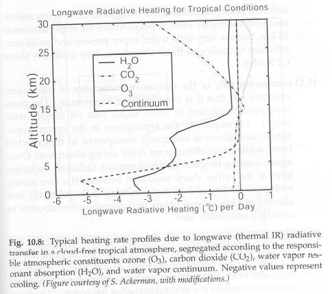
From Petty (2006)
Figure 2
And a set of graphs detailing the tropical condition for temperature, pressure, density and GHG concentrations:
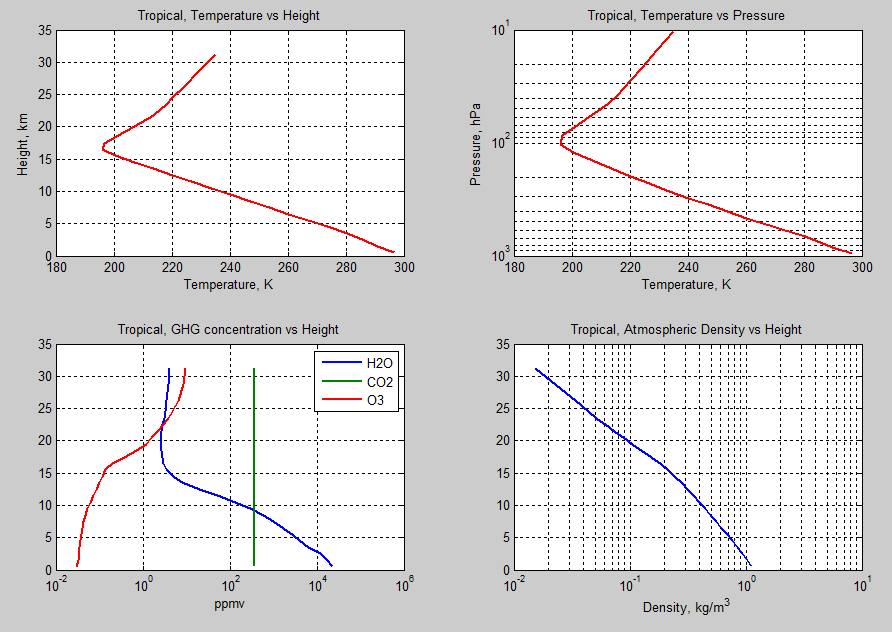
Figure 3 – Click to enlarge
Now some comparisons of the overall heating rates for 3 different profiles:
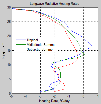
Figure 4
Here is a textbook comparison:
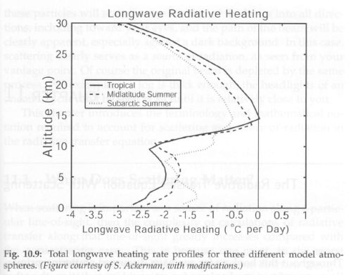
From Petty (2006)
Figure 5
So we can see that the MATLAB model created here from first principles and using the HITRAN database of absorption and emission lines is quite close to other calculated standards.
In fact, the differences are small except in the mid-stratosphere and we may find that this is due to slight differences in the model atmosphere used, or as a result of not using the Voigt profile (this is an important but technical area of atmospheric radiation – line shapes and how they change with pressure and temperature in the atmosphere – see for example Part Eight – CO2 Under Pressure).
Pekka Pirilä has been running this MATLAB model as well, has helped with numerous improvements and has just implemented the Voigt profile so we will shortly find out if the line shape is a contributor to any differences.
For reference, here are the profiles of the other two conditions shown in figure 4: Midlatitude summer & Subarctic summer:
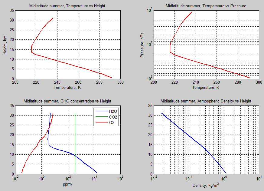
Figure 6 – Click to enlarge
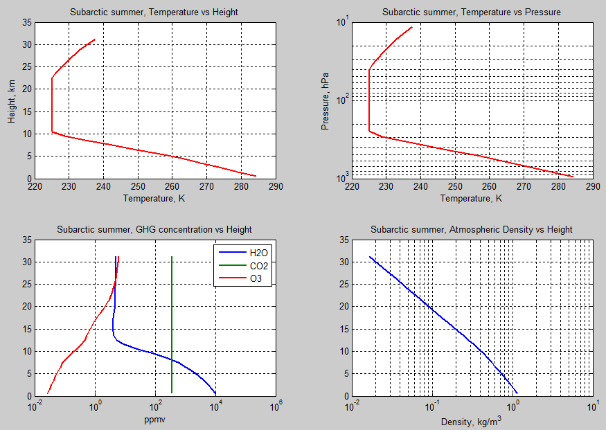
Figure 7 – Click to enlarge
Related Articles
Part One – some background and basics
Part Two – some early results from a model with absorption and emission from basic physics and the HITRAN database
Part Three – Average Height of Emission – the complex subject of where the TOA radiation originated from, what is the “Average Height of Emission” and other questions
Part Four – Water Vapor – results of surface (downward) radiation and upward radiation at TOA as water vapor is changed
Part Five – The Code – code can be downloaded, includes some notes on each release
Part Six – Technical on Line Shapes – absorption lines get thineer as we move up through the atmosphere..
Part Seven – CO2 increases – changes to TOA in flux and spectrum as CO2 concentration is increased
Part Eight – CO2 Under Pressure – how the line width reduces (as we go up through the atmosphere) and what impact that has on CO2 increases
Part Nine – Reaching Equilibrium – when we start from some arbitrary point, how the climate model brings us back to equilibrium (for that case), and how the energy moves through the system
Part Ten – “Back Radiation” – calculations and expectations for surface radiation as CO2 is increased
Part Eleven – Stratospheric Cooling – why the stratosphere is expected to cool as CO2 increases
Part Thirteen – Surface Emissivity – what happens when the earth’s surface is not a black body – useful to understand seeing as it isn’t..
References
AFGL atmospheric constituent profiles (0.120 km), by GP Anderson et al (1986)
A First Course in Atmospheric Radiation, Grant Petty, Sundog Publishing (2006)
The data used to create these graphs comes from the HITRAN database.
The HITRAN 2008 molecular spectroscopic database, by L.S. Rothman et al, Journal of Quantitative Spectroscopy & Radiative Transfer (2009)
The HITRAN 2004 molecular spectroscopic database, by L.S. Rothman et al., Journal of Quantitative Spectroscopy & Radiative Transfer (2005)


“…the differences are small except in the mid-stratosphere and we may find that this is due to…”
May be due to the height of your profile ( appears to be around 32km ).
I found that height of the profile makes a difference with other radiative models. When a profile is cut off at ~30km, that means in the model, there is zero CO2 above that level and some below leading to intense cooling. In reality, CO2 tapers off more slowly up to the top of the homosphere ( around 100km ), leading to less negative heating rates in the stratosphere.
https://scienceofdoom.files.wordpress.com/2010/01/co2-h2o-atmospheric-concentration.png?w=750&h=375
When you get time, I suggest using a profile that extends closer to 100km ( about the top of the homosphere ) to test any difference. ( may have to make some assumptions based for mesospheric temperatures ).
I have extended now the calculation to the pressure level of 1 Pa (73 km, the top layer is from 47.7 km to 73.0 km or in terms of pressure from 1 Pa to 60.0 Pa) using the Voigt profile. The case is not the one discussed in this Part 12, but close to that of Part 11. In that case the temperature of the top layer is as high as 273 K for 280 ppm CO2 and no other GHG’s. The temperature keeps now on rising almost linearly up to the top layer. The case is, however, not fully realistic.
The value 273 K was actually obtained with the Lorentz profile, Voigt profile gives 265.5 K.
Doubling the CO2 concentration lowers the temperature of the top layer by 17.8 K to 247.7 K, while the surface temperature goes up from 279.30 K to 281.45 K, i.e. by 2.15 K. I emphasize again that the model is not fully realistic even for clear sky conditions.
The concentration of CO2 vs Height is depicted as constant at all altitudes, to the limit of the graph. Is this physically true, or a model assumption?
Earlier I had asked about how quickly an automobile’s tailpipe CO2 might appear in the stratosphere, relative to that of a high-flying jet, and the answer seemed to be on a timescale of years, perhaps decades. So I wonder if there is a concentration gradient near the surface, where humans and others generate CO2, that quickly becomes a constant with height, or does it mix so rapidly that this is not observed?
If a volcano sent a large plume of CO2 convectively into the stratosphere, which then spread around the world by stratospheric winds (like the dust from Krakatoa) how quickly would constant CO2 concentration be re-established in the whole atmosphere, and until then, what is the net effect on the earth’s temperature due to CO2 changes of distribution alone? Large? Modest? Negligible?
JohnBoy,
It isn’t a topic I have researched.
Have a look at Vertical and meridional distributions of the atmospheric CO2 mixing ratio between northern midlatitudes and southern subtropics, Machida et al, JGR, 2003.
As well as graphs and discussions of that piece of research it seems there are many references that could be used as a starting point.
Other commenters might have more to add.
That paper seems to discuss only troposphere but the same group has studied also stratosphere. Google finds the paper “Carbon dioxide variations in the stratosphere over Japan, Scandinavia and Antarctica” by Aoki et al. but gives a link too complex for copying.
That paper tells that the stratospheric CO2 concentration does not depend on the altitude over the range 20-35 km and has been consistently about 5 ppm lower than the concentration in troposphere. The transition in the concentration seems to take place between 10 and 20 km.
The measurements have been made by balloons ans are therefor limited to altitudes up to 35 km.
There’s enough mixing in the stratosphere to prevent the difference in concentration from growing. The mixing continues even higher up in mesosphere. Above 100 km diffusion dominates and the concentration of heavier molecules like CO2 decreases with altitude. With pure diffusion each type of molecule has its own exponential rate of decrease with altitude.
I repeated the calculation using Voigt profile at pressures below 25 hPa (the results are the same to a few parts in 1000 when the limit is 10 hPa) allowing the altitude reach 85 km.
The tropical heating rate up to 30 km looks like this. It seems to agree with SoD’s calculation up to 25 km but drop much more slowly above 25 km. The upper part of the range of agreement is based on the Voigt profile. Thus it makes little difference at these altitudes.
Including the whole range up to 85 km is like this. The topmost part above 70 km is probably influenced strongly by the cut-off of the calculation at 85 km.
Here we see that the profile has little effect up to 40 km, but very much at the highest levels.
The results should not be taken at face value, because the frequency grid is too sparse to give reliable results. In particular with Lorentz profile all peaks are probably missed at lowest pressures. The same may apply to the highest point with Voigt profile, where my cutoffs may be too strict.
Increasing the number of frequencies makes a big difference at highest altitudes. Changing dv from 1 1/cm to 0.1 1/cm produced this.
Lorentz profile leads now to a more regular behavior. Changes are significant also for the Voigt profile. I’ll try also dv=0.01 1/cm, but that starts to get slow.
Now I have the results for Voigt profile with dv=0.01 1/cm. That calculation took about 5 hours. The results tell that small dv is important in mesosphere (50-80 km) and has some effect in the upper stratosphere as well.
This is the temperature profile of the tropical standard atmosphere that’s used in the calculation.
I reran the 3 atmospheric profiles shown in figure 4 with 3 isotopologues instead of just the main, and compared the heating rates. The differences are small, here shown as a percentage of the originally calculated heating rates:
The isotope fractions for water vapor: 99.73%, 0.20%, 0.04%
For CO2: 98.42%, 1.11%, 0.39%
For Ozone: 99.29%, 0.400%, 0.2%
The reason why the 2nd and 3rd might have more of an impact than indicated by their percentages is that many of their absorption lines are in different places to the main isotopologue – and so are absorbing in wavelengths with little absorption from other molecules.
I also checked the TOA OLR and the DLR and these are identical, which implies that they aren’t necessary for most simulation runs. The time taken was 16 minutes for 3 isotopologues (x 3 molecules) vs 6 minutes for a run which only used the main one (for each of the 3 molecules).
[…] « Visualizing Atmospheric Radiation – Part Twelve – Heating Rates […]
[…] Part Twelve – Heating Rates – heating rate (‘C/day) for various levels in the atmosphere – especially useful for comparisons with other models. […]
[…] Part Twelve – Heating Rates – heating rate (‘C/day) for various levels in the atmosphere – especially useful for comparisons with other models. […]
[…] Part Twelve – Heating Rates – heating rate (‘C/day) for various levels in the atmosphere – especially useful for comparisons with other models. […]
[…] Part Twelve – Heating Rates – heating rate (‘C/day) for various levels in the atmosphere – especially useful for comparisons with other models. […]
[…] Part Twelve – Heating Rates – heating rate (‘C/day) for various levels in the atmosphere – especially useful for comparisons with other models. […]
[…] Part Twelve – Heating Rates – heating rate (‘C/day) for various levels in the atmosphere – especially useful for comparisons with other models. […]
[…] 2013/01/30: TSoD: Visualizing Atmospheric Radiation – Part Twelve – Heating Rates […]
I have an old paper by Plass, Amer. Jour. Of Physics, 303(24), 1956 that I dug up long ago to understand radiation and IR gases in the atmosphere. His heating curves, Fig 9, are quite similar to yours but extend higher into the atmosphere. The plots show that above about 25 km cooling increases with increases in CO2 concentration as one would expect once the densities drop to the point where the IR can escape freely.
He also arrives at an increase in downward flux of about 8 W/m^2, for a doubling of CO@, about four times the modern estimate. This is probably due to the poor quality of spectral data available, particularly the lack of data for H2O. He also shows in Fig 8 (upwards and downwards fluxes for three CO2 concentrations), that the flux change is entirely due to the 12-14 um and 16-18um bands, the 14-15 um band being saturated.
It would be interesting if you could reproduce his plots but with the modern spectral data. If you don’t have access to his paper I’d be happy to send you a scan of the two figures.
Your Figs 1 and 4 show a tropical tropospheric hotspot but Fig 5 doesn’t. Both Lindzen and Spencer point out that it is not observed in the ballon or satellite data. What is the source of the hotspot in your calculations?
FWIF, here’s a link:
http://ajp.aapt.org/resource/1/ajpias/v24/i5/p303_s1
http://scitation.aip.org/getpdf/servlet/GetPDFServlet?filetype=pdf&id=AJPIAS000024000005000303000001&idtype=cvips&doi=10.1119/1.1934220&prog=normal
As for the hotspot, doubling CO2 imposes close to zero change in the radiative cooling rate for any given level in the troposphere. ( Seems paradoxical until reflecting that it is the accumulation of energy for the troposphere as a whole that implies warming ).
Further, the hotspot appears in models for other forcings ( reducing albedo, increasing solar, etc. )
This implies that the hotspot is arising from modeled atmospheric response to energy increase. These other processes are parameterized, of course.
The failure of the models in this respect represents a serious error in the parameterizations which probably doesn’t get enough attention. This is no surprise, of course. Atmospheric motion is non-linear and not accurately represented by parameterization ( if it were, we wouldn’t need any meteorologists ).
Climate Weenie,
A tropical hot spot means that the temperature increases faster in the upper troposphere than near the surface. By definition that means a decrease in the lapse rate. But the average relative humidity in the tropical atmosphere above 10 km is less than 20%. I’m not sure why, if the RH remains that far below saturation, the lapse rate should decrease.
DeWitt –
I think that’s part of the failing of the parameterizations.
Were the lapse rate to actually decrease, that would imply less convection, meaning less heating reaching the upper troposphere (and less moisture).
Tropical convection is dominated by the ITCZ. But the ITCZ arises from air mass motion – non-linear dynamics – which are not well parameterized.
What DeWitt writes is correct, but perhaps it doesn’t emphasize enough the fact that this post discusses issues that have essentially nothing to do with a hotspot. None of the figures tells anything about that or is in any obvious way related to that.
This post tells about the role of IR in the local energy balance at various altitudes. The atmosphere is assumed to follow one of the AFGL standard atmospheres, that’s assumed not calculated. The only thing that’s calculated is the IR emission and absorption that results from the assumed atmospheric profiles under clear sky conditions.
In troposphere the imbalance of the IR terms is compensated by SW absorption and convection, in stratosphere by SW absorption alone.
Climate Weenie,
The ITCZ is not something that dominates the tropical convection, it might be more correct to say that the tropical convection forces the existence of ITCZ. ITCZ represents the return flow of air when moist warm air rises as the uplift part of the Hadley cells. The reduced lapse rate is the consequence of this moist uplift, which is perhaps the most important driver of the global circulation. It drives almost everything, nothing drives it (except the solar heating of tropics).
Pekka, the point about the ‘hotspot’ is that, as you note, it’s not a function of radiative forcing from increased CO2, since CO2 doubling doesn’t change the cooling rate very much at all.
Rather the hotspot is predicted by the parameterizations of other processes ( probably convection ) and the lack of the hotspot appearance means the convection parameterization is likely quite erroneous.
The parameterization is wrong regardless of the source of the convection.
I was ready to dismiss the convection forces convergence argument until I reflected that hurricanes represent mutual feedback between convergence and convection – the inflow enhances convection while the convection ( and subsequent outflow aloft ) enhance converging inflow. The same probably occurs with the ITCZ – mutual feedback.
Still, ‘solar heating’ as theory runs into problems explaining why the ITCZ remains north of the equator year round in the Atlantic and the Eastern Pacific.
Further, tracing individual polar air masses by examining the total precipitable water demonstrates that polar air masses, greatly modified, do make their way to the equator and the instrusion of these air masses do show up as waves in the ITCZ.
That’s one problem I have with the ‘Hadley Cell’, which is not actually observed in nature. The ‘Cells’ don’t allow for air mass exchange across them. A better model, it seems to me, is that there is no such thing as the ‘sub tropical jet’, Hadley Cell, Ferrel Cell and the like, but polar air masses which spill underneath the baroclinic waves as part of the global circulation. There is an equatorial low in association with the ITCZ, but there is a large contribution of the convergence of polar air masses in driving the convection in the conditionally unstable air of the deep tropics.
[…] (air force geophysics lab) atmospheres. A description of some of them can be seen in Part Twelve – Heating Rates (note […]