The earth’s surface is not a black-body. A blackbody has an emissivity and absorptivity = 1.0, which means that it absorbs all incident radiation and emits according to the Planck law.
The oceans, covering over 70% of the earth’s surface, have an emissivity of about 0.96. Other areas have varying emissivity, going down to about 0.7 for deserts. (See note 1).
A lot of climate analyses assume the surface has an emissivity of 1.0.
Let’s try and qualify the effect of this assumption.
The most important point to understand is that if the emissivity of the surface, ε, is less than 1.0 it means that the surface also reflects some atmospheric radiation.
Let’s first do a simple calculation with nice round numbers.
Say the surface is at a temperature, Ts=289.8 K. And the atmosphere emits downward flux = 350 (W/m²).
- If ε = 1.0 the surface emits 400. And it reflects 0. So a total upward radiation of 400.
- If ε = 0.8 the surface emits 320. And it reflects 70 (350 x 0.2). So a total upward radiation of 390.
So even though we are comparing a case where the surface reduces its emission by 20%, the upward radiation from the surface is only reduced by 2.5%.
Now the world of atmospheric radiation is very non-linear as we have seen in previous articles in this series. The atmosphere absorbs very strongly in some wavelength regions and is almost transparent in other regions. So I was intrigued to find out what the real change would be for different atmospheres as surface emissivity is changed.
To do this I used the Matlab model already created and explained – in brief in Part Two and with the code in Part Five – The Code (note 2). The change in surface emissivity is assumed to be wavelength independent (so if ε = 0.8, it is the case across all wavelengths).
I used some standard AFGL (air force geophysics lab) atmospheres. A description of some of them can be seen in Part Twelve – Heating Rates (note 3).
For the tropical atmosphere:
- ε = 1.0, TOA OLR = 280.9 (top of atmosphere outgoing longwave radiation)
- ε = 0.8, TOA OLR = 278.6
- Difference = 0.8%
Here is the tropical atmosphere spectrum:
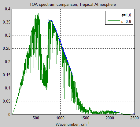
Figure 1
We can see that the difference occurs in the 800-1200 cm-1 region (8-12 μm), the so-called “atmospheric window” – see Kiehl & Trenberth and the Atmospheric Window. We will come back to the reasons why in a moment.
For reference, an expanded view of the area with the difference:
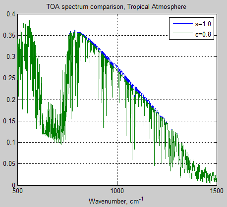
Figure 2
Now the mid-latitude summer atmosphere:
- ε = 1.0, TOA OLR = 276.9
- ε = 0.8, TOA OLR = 272.4
- Difference = 1.6%
And the mid-latitude winter atmosphere:
- ε = 1.0, TOA OLR = 227.9
- ε = 0.8, TOA OLR = 217.4
- Difference = 4.6%
Here is the spectrum:
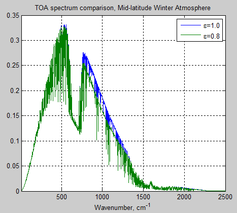
Figure 3
We can see that the same region is responsible and the difference is much greater.
The sub-arctic summer:
- ε = 1.0, TOA OLR = 259.8
- ε = 0.8, TOA OLR = 252.7
- Difference = 2.7%
The sub-arctic winter:
- ε = 1.0, TOA OLR = 196.8
- ε = 0.8, TOA OLR = 186.9
- Difference = 5.0%
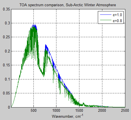
Figure 4
We can see that the surface emissivity of the tropics has a negligible difference on OLR. The higher latitude winters have a 5% change for the same surface emissivity change, and the higher latitude summers have around 2-3%.
The reasoning is simple.
For the tropics, the hot humid atmosphere radiates quite close to a blackbody, even in the “window region” due to the water vapor continuum. We can see this explained in detail in Part Ten – “Back Radiation”.
So any “missing” radiation from a non-blackbody surface is made up by reflection of atmospheric radiation (where the radiating atmosphere is almost at the same temperature as the surface).
When we move to higher latitudes the “window region” becomes more transparent, and so the “missing” radiation cannot be made up by reflection of atmospheric radiation in this wavelength region. This is because the atmosphere is not emitting in this “window” region.
And the effect is more pronounced in the winters in high latitudes because the atmosphere is colder and so there is even less water vapor.
Now let’s see what happens when we do a “radiative forcing” calculation – we will do a comparison of TOA OLR at 360 ppm CO2 – 720 ppm at two different emissivities for the tropical atmosphere. That is, we will calculate 4 cases:
- 360 ppm at ε=1.0
- 720 ppm at ε=1.0
- 360 ppm at ε=0.8
- 720 ppm at ε=0.8
And, at both ε=1.0 & ε=0.8 we subtract the OLR at 360ppm from OLR at 720ppm and plot both differenced emissivity results on the same graph:
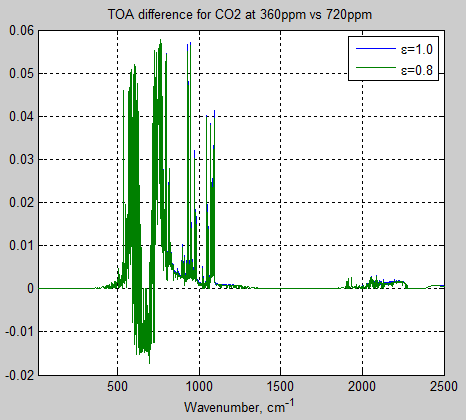
Figure 5
We see that both comparisons look almost identical – we can’t distinguish between them on this graph. So let’s subtract one from the other. That is, we plot (360ppm-720ppm)@ε=1.0 – (360ppm – 720ppm)@ε=0.8:
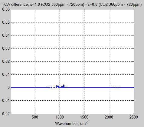
Figure 6 – same units as figure 5
So it’s clear that in this specific case of calculating the difference in CO2 from 360ppm to 720ppm it doesn’t matter whether we use surface emissivity = 1.0 or 0.8.
Conclusion
The earth’s surface is not a blackbody. No one in climate science thinks it is. But for a lot of basic calculations assuming it is a blackbody doesn’t have a big impact on the TOA radiation – for the reasons outlined above. And it has even less impact on the calculations of changes in CO2.
The tropics, from 30°S to 30°N, are about half the surface area of the earth. And with a typical tropical atmosphere, a drop in surface emissivity from 1.0 to 0.8 causes a TOA OLR change of less than 1%.
Of course, it could get more complicated than the calculations we have seen in this article. Over deserts in the tropics, where the surface emissivity actually gets below 0.8, water vapor is also low and therefore the resulting TOA flux change will be higher (as a result of using actual surface emissivity vs black body emissivity).
I haven’t delved into the minutiae of GCMs to find out what they assume about surface emissivity and, if they do use 1.0, what calculations have been done to quantify the impact.
The average surface emissivity of the earth is much higher than 0.8. I just picked that value as a reference.
The results shown in this article should help to clarify that the effect of surface emissivity less than 1.0 is not as large as might be expected.
Notes
Note 1: Emissivity and absorptivity are wavelength dependent phenomena. So these values are relevant for the terrestrial wavelengths of 4-50μm.
Note 2: There was a minor change to the published code to allow for atmospheric radiation being reflected by the non-black surface. This hasn’t been updated to the relevant article because it’s quite minor. Anyone interested in the details, just ask.
In this model, the top of atmosphere is at 10 hPa.
Some outstanding issues remain in my version of the model, like whether the diffusivity improvement is correct or needs improvement, and the Voigt profile (important in the mid-upper stratosphere) is still not used. These issues will have little or no effect on the question addressed in this article.
Note 3: For speed, I only considered water vapor and CO2 as “greenhouse” gases. No ozone was used. To check, I reran the tropical atmosphere with ozone at the values prescribed in that AFGL atmosphere. The difference between ε = 1.0 and ε = 0.8 was 0.7% – less than with no ozone (0.8%). This is because ozone reduces the transparency of the “atmospheric window” region.


[…] 2013/02/17: TSoD: Visualizing Atmospheric Radiation – Part Thirteen – Surface Emissivity […]
Modtran indicates a warming effect of 6 W/m2 by adding 0.0001% CO2 to a dry atmosphere?
High Emissivity of 1 ppm CO2!
http://claesjohnson.blogspot.com/2013/02/modtran-high-emissivity-of-1-ppm-co2.html
The attitude of that post makes no sense at all. Nobody can have any intuitive understanding on the size of the effect without some calculations. The basics of Modtran calculations are clear and easy enough to understand. This series of posts has discussed that from many different angles.
Claes Johnson just shows, how ignorant and unwilling to accept realities he is. He has the full explanation in front of him, but just decides to doubt it without any real argument, only the prejudices.
The post compares the Modtran results to the absorption spectrum for 1000 m of 1 ppm CO2 computed by Spectralcalc, which shows extreme sparsity of absorption away from the narrow interval 667-669, in contrast to a much wider interval of absorption computed by Modtran. What is the explanation for this?
Hockey Schtick.
For one the effective one atmosphere path length for the atmosphere is 8,000m, not 1,000m. A surface pressure of 101325 Pa is equal to 10328 kg/m². The average molecular weight of dry air is 0.0289465 kg/mole. At STP, that’s 7992 cubic meters/square meter or a path length of 7992m. We’re not at STP, but it’s a good approximation if you don’t want to subscribe to Spectralcalc to do a proper atmosphere path. The resolution of MODTRAN is only 2 cm-1because it uses a band model, not line-by-line, so the narrow lines get smeared together.
1 ppmv CO2 1000 m path
1 ppmv CO2 8000 m path
Total pressure 1013.25mbar
Temperature 288K
A band model does not necessarily work well over a wide range of concentrations as defining the bands may be optimized for more realistic cases. The low concentration case is, however, not particularly difficult to calculate, because the absorption at relatively low altitudes and high pressure are most important in that case.
I made a few tests with SoD’s model that’s well applicable to this task. It’s a line-by-line model and efficient for this case due to the dominance of well broadened lines.
For the AFGL midlatitude summer atmosphere the OLR at TOA for zero CO2 is 308.1 W/m^2 and for 1 ppm CO2 303.0 W/m^2, i.e. the forcing is 5.1 W/m^2 for this case.
For the midlatitude winter the forcing is 4.3 W/m^2, and for the tropic atmosphere 5.4 W/m^2.
Hockey Schtick,
Citing Claes Johnson won’t win you any points on serious climate blogs.
Did you actually go to the MODTRAN site and look at the spectra? At 1 ppmv, the effect of CO2 is still nearly linear and it absorbs very strongly. A reduction in emission to space of 6 W/m² for going from zero to one ppmv CO2 is quite reasonable.
I suggest you go to the MODTRAN site set the water vapor scale and CO2, CH4, tropospheric ozone and stratospheric ozone scale to zero. Set the atmosphere to 1976 US Standard Atmosphere, no clouds or rain and the sensor position to 100 km looking down. Then calculate spectra for different concentrations of CO2 and actually look at the spectra. Even better, calculate the spectra for 0.01, 0.02, 0.05, 0.1, 0.2 … 200,500 ppmv CO2 and plot the absolute value of the difference in emission from 0 ppmv CO2 vs log CO2. You might actually learn something.
I set the parameters as you suggested, comparing the spectra for 0 ppm CO2 to 1 ppm CO2 and find the Modtran graph shows a much wider absorption interval for CO2 between ~600-700 nm as compared to Spectracalc, which shows extreme sparsity of absorption away from the narrow interval of 667-669 nm. What is the explanation for this?
Hockey Schtick,
I clicked on the wrong reply link so my reply is above if you’re viewing this threaded rather than chronological.
Thanks for your reply.
What does Spectralcalc determine as the reduction in emission in W/m2 for 8000 m path length for going from 0 to 1 ppm CO2?
Hockey Schtick,
That data is only available to subscribers. Spend $49 for a 30 day subscription and find out. Then you can also calculate a proper atmospheric path.
Here’s an analysis done with Spectralcalc which determines doubling of current CO2 levels could only raise surface temperature < 0.2 C
http://climateclash.com/g4-a-subscriber-paper-request-for-review/
Using SpectralCalc or any other valid source as input does not lead to correct results by itself. The input must also be used correctly. This series of 13 posts (so far) has approached that same problem and done it basically correctly. The results are totally different, because Bryce Johnson did not do much correctly.
It’s not really productive to go through all the erroneous calculations that somebody has made. It’s much better to take the correct approach and work through that. It’s immediately clear that Bryce Johnson’s calculation do not include those absolutely essential ingredients that are used by SoD in his model. As SoD’s model is openly available, everyone is free to study it. Any specific questions will certainly be answered by him or somebody else who has already studied the model well enough to understand it.
“It’s immediately clear that Bryce Johnson’s calculation do not include those absolutely essential ingredients that are used by SoD in his model.”
What specifically would those missing “absolutely essential ingredients” be? What would be your top 3 missing ingredients?
It’s not right to start by asking what’s missing, when a better question is, why should that calculation have any relevance at all.
The correct calculation must have the general structure that
– it is based on a realistic atmospheric profile for pressure, temperature, and concentrations of vapor and CO2,
– it takes into account absorption and emission at different altitudes using a multi-layer model (or some comparable approach)
– it considers each wavelength separately either as a band model or as a line-by-line model
Bryce Johnson uses SpetralCalc for the third point but neglects the others. He makes explicitly wrong claims on the importance of related issues.
According to the SpectraCalc documentation, “Each model atmosphere contains temperature, pressure and gas concentrations at all altitudes.” which means your first two “essential ingredients” are already included.
As you note, SpectraCalc is a line-by-line calculation, which means your 3rd top “essential ingredient” is already included.
Do you have any more missing “essential ingredients”?
[Sorry Pekka, just retrieved from the spam queue]
I’m not interested in spending much time with an article that’s clearly wrong and that justifies it’s calculations with explicitly wrong claims. By these explicitly wrong claims I mean all those statements that some issues don’t matter. Many of those issues matter very much, and taking them into account is essential for getting meaningful answers.
Leaving out of discussion the other essential ingredients that I mentioned means that the calculation is not a calculation of the Earth atmosphere or of the warming influence of the CO2 on the Earth. As it’s not such a calculation, it’s not a calculation of much interest. The best way forward is not to try to correct that calculation but to take a fresh start by looking at the case we are interested in, i.e. the real Earth atmosphere and see, how we can learn about that. This is the approach of this site. SoD is proceeding stepwise and brings up issues that are accessible to people that are not specialists. He has now covered the issues of the Bryce Johnson post, but done that correctly.
The Earth system is not that simple that anyone can just pick an idea and expect meaningful results. Following SoD requires some background understanding of physics, and it requires some work. He cannot make miracles and explain genuinely complex issues very simply, but his approach has shown that there’s a lot that can be learned with some background and with a reasonable effort.
Looking at a post like that of Bryce Johnson it’s enough for me to notice that
1) he does not do a calculation that takes into account all absolutely essential ingredients (one out of three is worth nothing)
2) he gets results that contradict very strongly calculations that are looking at the same questions more correctly
3) he does not justify his calculations by valid arguments and leaves actually very much totally without justification
This set of failures is very common. In particular the third is typical. The posts or “articles” describe some mathematical operation, but don’t even try to justify it’s relevance. It seems that the authors have decided to do some calculation without understanding at all what they are calculating. Then they just declare at the end that the calculation has proven something, in spite of the fact that they have calculated something totally different, something that doesn’t tell much about the issue they claim to have proven. This kind of work cannot usually be corrected, a new start is needed.
Hockey Schtick,
Your citing of Bryce Johnson is clear evidence of confirmation bias. You only accept things that confirm what you already believe. Years ago I thought that CO2 couldn’t possibly have a significant effect on the climate. But I did my homework and discovered that I had been wrong. But you need a solid grounding in Physical Meteorology and Atmospheric Radiative Transfer to understand why. As Feynman said, you should be most skeptical of things that confirm what you already believe. That’s the mark of a true skeptic.
Dewitt,
Do you understand that the RT calculated +3.7 W/m^2 from 2xCO2 is only a theoretical measurement?
I did not say I accept Bryce Johnson’s analysis – I am simply asking what, if anything, is problematic with it? So far, the only specific criticisms above do not apply.
So, please let us know specifically why you think Bryce Johnson’s SpectralCalc analysis is wrong.
Perhaps it tells something about BJ’s calculation that he messes totally up from the very beginning where he calculates solid angles. The numbers listed below equation (2) are false so badly that everyone should notice that without any calculation (the first one should be pi/4, the second one pi/2 and the last two should ad up to pi/4). This is not the most significant error for the outcome, but erring already on that tells about the quality of the work.
The calculation is basically not right, but it has enough content for expecting a result that’s closer to the correct one. The reason for the very small warming seems to be in the division by 10 of the effect as seen comparing in the Table 2 the lines Ratio to no-CO2 value to Ratio to total current atmosphere heat. That is explained in Assumptions by “The greenhouse contribution to total atmospheric heat is assumed to be ten percent. This is derived from the values indicated in Figures 2, 3 and 4 which are heat balances from the IPCC, the National Weather Service and from NASA.”. This is totally unjustified. It’s not surprising that the results are low, when the author divides the effect by 10 for totally spurious reasons.
What’s the point of doing calculations, when the author feels free to distort them like that.
So, you think that Bryce should have instead assumed 100% of total current atmospheric heat is contributed by the greenhouse effect, right?
He should have accepted that the calculation gives directly the correct value for the effect. All factors that limit the size of the effect are included in the calculation. Thus there’s no reason to reduce the effect by an additional factor of 1/10.
I really cannot figure out, what made him think that such an additional factor would be needed. That doesn’t make any sense at all.
1. Bryce’s assumption that 10% of total atmospheric heat is a result of the greenhouse effect is easily confirmed to be approximately correct by 33K/288K = 11.4%
2. He does not divide the effect by 1/10 as you claim.
a. He determines heat to the the atmosphere given 400 ppm vs. 800 ppm CO2 using SpectralCalc
b. determines the ratio of this to atm with no CO2
c. then determines the ratio to total atm heat
d. and determines the ratio to that at current CO2 level
e. takes the 4th root of the (d) ratio [given the T^4 relation in SB Law]
f. multiples global temp by this 4th root to obtain the new surface temp
Whether the estimate is correct or not doesn’t matter, because the share is taken into account in the calculation without any additional factors. Adding it once more means including it twice. If the factor is 1/10 he makes it to 1/100.
1. Bryce’s SpectralCalc calculations obviously do include the other sources of atmospheric heat other than the greenhouse effect, as confirmed by energy budget calculations
2. Another way of doing the calculation is to simply use the alleged greenhouse effect of 33K as the divisor instead of 288K
i.e. 33/244.64^.25 * 249.58^.25 = 33.166
33.166-33 = 0.166 = 0.17, i.e. the same temperature change calculated by Bryce.
There is absolutely no dividing by 10 in this calculation as you claim.
Thus, his assumptions are correct.
There’s no separate dividing, but why should that kind of division be added.
What I meant is that the calculation tells, how much absorption there is. If one mechanism is 10% then a direct calculation tells that it’s 10%, not that it were 100% and should be divided by 10 to make it 10%.
We have only one system. Every effect is there with it’s own strength, not by 10 times it’s strength or by 1/10 of its strength. Adding such extra divisions is totally wrong.
I emphasized that argument because adding arbitrarily extra factors is always wrong.
A separate issue is that the statement that
First of all it’s not clear what that sentence is supposed to mean. It seems ti be derived as ratio of some numbers found from those figures, but how could any numbers of these figures mean such a thing, whatever it’s supposed to mean. We can see from the Figure 2 that downwelling radiation from GHG’s is large. Similarly the total emission form surface is large. Neither of these numbers is 10% of any other quantity, they are rather more than 100% of the incoming or outgoing radiation.
Due to the GHE the Earth surface radiates about 65% more than the outgoing LW or the incoming SW when the albedo effect is taken into account. The whole difference is maintained by the GHE.
Hockey Schtick,
Step b is problematic for several reasons. The effect of CO2 isn’t linear, it’s logarithmic above 10 ppmv and approaches linearity below that. And there really is water vapor feedback on the down side because lowering the temperature will cause condensation and lower the specific humidity, further lowering the temperature because water vapor is also a ghg.
The rest of the steps are not the correct way to determine the temperature change necessary to restore radiative balance either. What you need to do to obtain a crude estimate is to calculate the entire spectrum looking down at the tropopause to avoid dealing with the stratosphere and integrate it. That gives you the total emitted power. Then change the CO2 and calculate the total emitted power again. Then change the surface temperature until the emitted power equals the emitted power before changing CO2. It’s crude because what you really need to do is recalculate the entire temperature and pressure profile to very high altitude when you change the surface temperature. MODTRAN won’t let you do that. It only changes the temperature and humidity, but not the atmospheric pressure and density below 11 km. So it’s really only good for small changes.
Using MODTRAN 1976 US standard atmosphere and starting at 375 ppmv CO2. The tropopause is at 11 km. Surface temp is 288.2K
Iout = 266.178 W/m² (100-1500 cm-1)
CO2 = 750 ppmv
Iout = 262.724 W/m²
water vapor pressure constant:
surface temperature = 289.15 K (+0.95)
Iout = 266.178 W/m²
relative humidity constant:
surface temperature = 289.56 K (+ 1.36)
Iout = 266.178 W/m²
CO2 = 0 ppmv
Iout = 293.778 K
water vapor pressure constant (physically extremely unrealistic)
surface temperature = 281.28 K (-6.92)
Iout = 266.178 W/m²
relative humidity constant
surface temperature = 278.12 K (-10.08)
Iout = 266.178 W/m²
Going to zero CO2 is highly problematic. The stratosphere would warm a lot requiring a larger decrease in surface temperature to restore radiative balance. Also, with a global average temperature that low, the entire planet would likely freeze over, substantially increasing albedo and lowering the temperature even further. So this result is sort of a back of the envelope calculation. I would be very surprised if the result using this process with Spectralcalc were substantially different. Using Spectralcalc is something of a PITA for this. The resolution is so high and there is a limit on the size of the data file requiring that the spectrum must be broken into segments. Determining the surface temperature offset is an iterative process so it takes a lot longer than using MODTRAN.
Let’s dispense with the problems of comparing 400 or 800 ppm to 0 ppm CO2 and stick with “smaller changes”
1. We assume the entire GHE with 400 ppm CO2, current water vapor, and including all feedbacks is causing a total of 33K warming
2. We assume the SpectralCalc calculations of 244.64 W/m2 heat to the atmosphere including all sources is correct for 400 ppm CO2, and that this is causing the 33K net increase in surface temperature
3. We assume the SpectralCalc calculations of 249.58 W/m2 heat to the atmosphere including all sources is correct for 800 ppm CO2
4. Thus, the new greenhouse effect is calculated as
33/244.64^.25 * 249.58^.25 = 33.166 K
33.166 – 33 = 0.166 C net warming from doubled CO2
While not claiming this is perfect, I don’t believe this calculation is off by a factor of 10.
Furthermore, even if it was off by a factor of 10, that would mean climate sensitivity to CO2 increase alone is 1.7 C, about 70% higher than even the IPCC claims of 1 C from doubled CO2 alone.
#2 clarified:
2. We assume the SpectralCalc calculations of 244.64 W/m2 heat to the atmosphere including all sources is correct for 400 ppm CO2, and that the GHE contribution is causing the 33K net increase in surface temperature to 288K
The effect is not relative to 33K, it’s relative to 288K. That’s the temperature that is raised to the fourth power.
I realized only now that your earlier comment was also referring to the factor of 33/288 or something like that as contributing to the argument. That’s not correct. Nothing in the calculation of the temperature change due to doubling of CO2 refers in any way whatsoever to the case of zero CO2.
The change in temperature is ((249.58/244.64)^0.25-1)*288K = 1.44K for the numbers you present.
Hockey Schtick,
Look at it from the other direction. And increase of 0.16 K from 288.2 to 288.36 increases surface emission from 391.16 W/m² to 392.03 W/m² or a difference of 0.87 W/m² assuming a surface emissivity of 1, less at lower emissivity. How does this possibly square with Johnson’s calculated increase in radiation of 4.94 W/m². Answer: It doesn’t. Johnson’s calculation is incorrect. As Pekka pointed out, an increase of 4.94 W/m² at 288 K requires a temperature increase of 1.44 K.
Thanks for your comments. I see your point and agree that Bryce Johnson’s analysis is flawed.
Perhaps Professors of Applied Mathematics don’t understand the scientific method used in physics.
The argument from incredulity might appeal to an audience uninterested in science and perhaps this is his target.
But you would expect the professor to understand maths?
And so, if the intensity, Iout(v) = Iin(v).exp(-τ(v))
Where Iin(v) = input intensity as a function of wavenumber, v, and τ(v) = optical thickness as a function of wavenumber we can say that the Professor is correct in his argument from incredulity if, and only if, there is only one optical thickness that is valid across all absorbing wave numbers.
Once we realize that there are many different optical thicknesses for different wave numbers then, for the mathematicians we can simplify the real problem a little, and take n different bands, and assume we have constant input intensity across these bands – just to make life simple for the mathematicians –
Iout = Iin./n.Σexp(-τn)
And now we ask ourselves, what brain-crunchingly difficult solution could we find where Prof. Johnson’s argument from incredulity was not correct?
Thinking, thinking.. Many days pass.. Finally..
If τi ≠ τj
Wow. That was a challenging maths problem and I am amazed I managed to come up with the solution.
My comment above was in reference to Hockey Schtick’s original comment of February 19, 2013 at 2:47 am, re Claes Johnson’s article. Seeing as we have two gentleman of the same surname under discussion..
I thought the emissivity of water is more like about 0.99.
It gets a little complicated due to the fact that we need the value through all angles.
See Emissivity of the Ocean – many experiments and studies on this unexciting but essential subject.