The Science of Doom

“Blah blah blah” vs Equations

January 30, 2012 by scienceofdoom

It is not surprising that the people most confused about basic physics are the ones who can’t write down an equation for their idea.

The same people are the most passionate defenders of their beliefs and I have no doubts about their sincerity.

I’ll meander into what it is I want to explain..

I found an amazing resource recently – iTunes U short for iTunes University. Now I confess that I have been a little confused about angular momentum. I always knew what it was, but in the small discussion that followed The Coriolis Effect and Geostrophic Motion I found myself wondering whether conservation of angular momentum was something independent of, or a consequence of, linear momentum or some aspect of Newton’s laws of motion.

It seemed as if conservation of angular momentum was an orphan of Newton’s three laws of motion. How could that be? Perhaps this conservation is just another expression of these laws in a way that I hadn’t appreciated? (Knowledgeable readers please explain).

Just around this time I found iTunes U and searched for “mechanics” and found the amazing series of lectures from MIT by Prof. Walter Lewin. A series of videos. I recommend them to anyone interested in learning some basics about forces, motion and energy. Lewin has a gift, along with an engaging style. It’s nice to see chalk boards and overhead projectors because they are probably no more in use (? young people please advise).

These lectures are not just for iPhone and iTunes people – here is the weblink.

The gift of teaching science is not in accuracy – that’s a given – the gift is in showing the principle via experiment and matching it with a theoretical derivation, and “why this should be so” and thereby producing a conceptual idea in the student.

I haven’t got to Lecture 20: Angular Momentum yet, I’m at about lecture 11. It’s basic stuff but so easy to forget (yes, quite a lot of it has been forgotten). Especially easy to forget how different principles link together and which principle is used to derive the next principle.

What caught my attention for the purposes of this article was how every principle had an equation.

For example, in deriving the work done on an object, Lewin integrates force over the distance traveled and comes up with the equation for kinetic energy.

While investigating the oscillation of a mass on a spring, the equation for its harmonic motion is derived.

Every principle has an equation that can be written down.

Over the last few days, as at many times over the past two years, people have arrived on this blog to explain how radiation from the atmosphere can’t affect the surface temperature because of blah blah blah. Where blah blah blah sounds like it might be some kind of physics but is never accompanied by an equation.

Here’s the equation I find in textbooks.

Energy absorbed from the atmosphere by the surface, E_a:

E_a = αR_L↓ ….[eqn 1]

where α = absorptivity of the surface at these wavelengths, R_L↓ = downward radiation from the atmosphere

And this energy absorbed, once absorbed, is indistinguishable from the energy absorbed from the sun. 1 W/m² absorbed from the atmosphere is identical to 1 W/m² absorbed from the sun.

That’s my equation. I have provided six textbooks to explain this idea in a slightly different way in Amazing Things we Find in Textbooks – The Real Second Law of Thermodynamics.

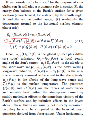
It’s also produced by Kramm & Dlugi, who think the greenhouse effect is some unproven idea:

Now the equation shown is a pretty simple equation. The equation reproduced in the graphic above from Kramm & Dlugi looks a little more daunting but is simply adding up a number of fluxes at the surface.

Here’s what it says:

Solar radiation absorbed + longwave radiation absorbed – thermal radiation emitted – latent heat emitted – sensible heat emitted + geothermal energy supplied = 0

Or another way of thinking about it is energy in = energy out (written as “energy in – energy out = 0“)

Now one thing is not amazing to me – of the tens (hundreds?) of concerned citizens commenting on the many articles on this subject who have tried to point out my “basic mistake” and tell me that the atmosphere can’t blah blah blah, not a single one has produced an equation.

The equation might look something like this:

E_a = f(α,T_atm-T_sur).R_L↓ ….[eqn 2]
where T_atm = temperature of the atmosphere, T_sur = temperature of the surface

With the function f being defined like this:

f(α,T_atm-T_sur) = α, when T_atm ≥ T_sur and

f(α,T_atm-T_sur) = 0, when T_atm < T_sur

In English, it says something like energy from the atmosphere absorbed by the surface = 0 when the temperature of the atmosphere is less than the temperature of the surface.

I’m filling in the blanks here. No one has written down such ridiculous unphysical nonsense because it would look like ridiculous unphysical nonsense. Or perhaps I’m being unkind. Another possibility is that no one has written down such ridiculous unphysical nonsense because the proponents have no idea what an equation is, or how one can be constructed.

My Prediction

No one will produce an equation which shows how no atmospheric energy can be absorbed by the surface. Or how atmospheric energy absorbed cannot affect internal energy.

This is because my next questions will be:

Please supply a textbook or paper with this equation
Please explain from fundamental physics how this can take place

My Challenge

Here’s my challenge to the many people concerned about the “dangerous nonsense” of the atmospheric radiation affecting surface temperature –

Supply an equation.

If you can’t, it is because you don’t understand the subject.

It won’t stop you talking, but everyone who is wondering and reads this article will be able to join the dots together.

The Usual Caveat

If there were only two bodies – the warmer earth and the colder atmosphere (no sun available) – then of course the earth’s temperature would decrease towards that of the atmosphere and the atmosphere’s temperature would increase towards that of the earth until both were at the same temperature – somewhere between the two starting temperatures.

However, the sun does actually exist and the question is simply whether the presence of the (colder) atmosphere affects the surface temperature compared with if no atmosphere existed. It is The Three Body Problem.

My Second Prediction

The people not supplying the equation, the passionate believers in blah blah blah, will not explain why an equation is not necessary or not available. Instead, continue to blah blah blah.

Posted in Basic Science, Commentary | 455 Comments »

The Coriolis Effect and Geostrophic Motion

January 15, 2012 by scienceofdoom

The coriolis effect isn’t the easiest thing to get your head around, but it is an essential element in understanding the large scale motions of the atmosphere and the oceans.

If you roll a ball along a flat frictionless surface it keeps going in the same direction. This is because objects that have no forces on them continue in the same direction at the same speed. (The combination of direction and speed is known as velocity, which is a vector. A vector consists of a magnitude (e.g. speed) and a direction).

Well, that statement was not strictly true – because it wasn’t specific enough.

If you get onto a merry go round and launch your same ball in one direction you observe it move away in a curved arc. But someone above the merry go round, perhaps someone who had climbed up a pole and was looking down, would observe the ball moving in a straight line.

It’s all about frames of reference.

Now we live on planet that is rotating so we have to consider the “merry go round” effect.

There are two approaches for a mathematical basis (and we will keep the maths separated):

consider everything from an inertial frame – as if all motion was viewed from space (note 1)
consider everything from the surface of the planet

If we considered everything from space then the problem would actually be more difficult. On the plus side thrown balls would go in a straight line (as normal). On the minus side the boundaries of the oceans, mountains and everything else important would be constantly on the move and we would need mathematical trickery beyond most people’s comprehension.

So everyone goes for option b – consider motion from the surface of the planet. This means the frame of reference is constantly on the move.

Coriolis

The excellent Atmosphere, Ocean and Climate Dynamics by Marshall & Plumb (2008) comes with a number of accompanying web pages most of which have some videos.

See GFDLab V: Inertial Circles – visualizing the Coriolis force for some detail and the video link, or click on the image below for the video link:

Figure 1 – Click for the video

the left hand video is the inertial frame of reference – stationary camera
the right hand video is the rotational frame of reference – the camera is moving with the turntable

This is the best video I have found for making clear what happens in a rotating frame.

With some relatively simple maths, the equations of motion in an inertial frame get transformed into a rotating frame of reference.

Two new terms get introduced:

the Coriolis acceleration = “stuff appears to veer off to the side as far as I can tell” effect
centrifugal acceleration = “things get thrown outwards like on a merry-go-round that goes very fast” effect

The centrifugal acceleration is not so significant, just a slight modifier of magnitude and direction to the very strong gravitational effect. But the Coriolis effect is very significant.

Now the Coriolis effect is easy to demonstrate on a rotating table, but we live on a rotating sphere and so there are some complexities that require the use of vector maths to calculate.

Mathematically it is easy to show that the Coriolis effect is modified by a factor relating to latitude. Specifically the effect is multiplied by the sine of the latitude, which means that at the equator the Coriolis effect is zero (sin 0° = 0), and at 30° it is half the maximum (sin 30°=0.5) and at the poles it has the full effect (sin 90° = 1.0).

I found it difficult to come up with a conceptual model which helps readers see why this is so. Readers who have had to think about the effect of resolving forces and rotations into orthogonal directions might be able to provide a conceptual picture – so please add comment if you think so. (Note 2).

Some Maths

The Coriolis effect has to be seen in the light of the other terms in the equation of motion.

The intimidating version, for those not used to the equations of motion for fluids in a Lagrangian formulation (note 3):

Du/Dt + 1/ρ.∇p + ∇φ + fz x u = F_r …..[1]

where bold characters are vectors, z is the unit vector in the upward direction, u = velocity vector (u,v,w), φ = gravitational potential modified by the centrifugal force, ρ = density, p = pressure and f = Coriolis parameter.

And in not-quite-plain English, the change in velocity with time (following a moving parcel of fluid) plus pressure force plus gravitional force plus the coriolis force equals the frictional force (note that the terms are effectively for unit mass).

The Coriolis parameter:

f = 2Ω sinφ …..[2]

where Ω = the rotational speed of the earth (in radians/sec) = 2 π / (24*3600) = 7.3 x 10^-5 /s

And the simpler version in each local x,y,x direction with some simplifications applied (like the hydrostatic equilibrium approximation):

Du/Dt + 1/ρ . ∂p/∂x – f.v = F_x ….(local x-direction) …[3a]

Dv/Dt + 1/ρ . ∂p/∂y + f.u = F_y ….(local y-direction) …[3b]

1/ρ . ∂p/∂z + g = 0 ….(local z-direction) …[3c]

Geostrophic Balance and the Magnitude of the Coriolis Effect

Analysis of fluid flows is often carried out via non-dimensional ratios.

The Rossby number is the ratio of acceleration terms to the Coriolis force, and in the atmosphere at mid-latitudes is typically 0.1.

Another way of saying this is that the acceleration terms in equation 3 are a lot smaller than the Coriolis term. And in the free atmosphere (away from the boundary layer with the earth’s surface) the friction terms are negligible. This simplifies equation 3:

u_g = – 1/fρ . ∂p/∂y ….[4a]

v_g = 1/fρ . ∂p/∂x ….[4b]

With u_g, v_g defining the solution – geostrophic balance – to these simplified equations. This tells us that the E-W wind speed is proportional to the pressure change in the N-S direction, and the N-S wind speed is proportional to the pressure change in the E-W direction.

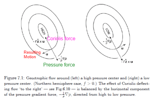
From Marshall & Plumb (2008)

Figure 2 – Colored text added

What might be surprising is the instead of the wind flowing from high to low pressure, it flows at right angles – along the lines of constant pressure.

So of course we have to ask whether these simplifications are justified..

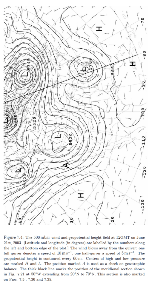
Here is a sample of the 500 mbar wind and geopotential height:

From Marshall & Plumb (2008)

Figure 3

We can see that the wind at 5oo mbar (about 5km high) is quite close to geostrophic balance.

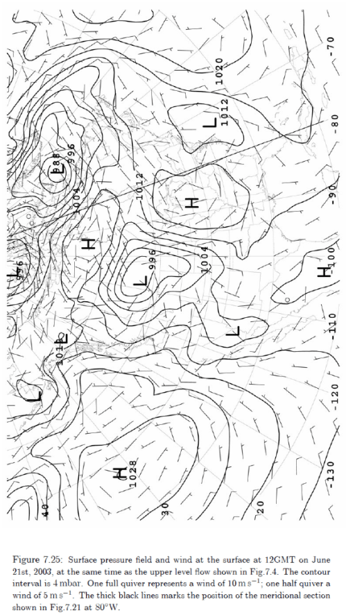
By contrast, if we look at surface winds:

From Marshall & Plumb (2008)

Figure 4

Here we see that the wind is flowing more across the pressure field from high to low pressure – this is because of the effect of friction at the surface. The friction term in equation 3 cannot be ignored when we want to calculate the motion near boundary layers.

Conclusion

This is just an interesting part of climate science. The large scale atmospheric and oceanic motion is fascinating and also necessary for understanding the science of climate.

Notes

Note 1: Even watching the planet from space is not an inertial frame of reference as the earth is rotating around the sun, and the sun is rotating around the center of the galaxy, etc, etc.. To avoid this article being a 100 page unfathomable treatise on rederiving the equations of motion, there are necessarily many simplifications, offered without caveat or explanation.

Note 2: The components of the Coriolis force on the surface of a sphere are calculated from Ω x u (where the “x” is the vector cross product, not “times”).

Ω x u = (0, Ωcosφ, Ωcosφ) x (u, v, w)

= (Ωcosφ.w – Ωsinφ.v, Ωsinφ.u, -Ωcosφ.u)

w is the vertical component of wind and is generally very small compared with horizontal components. So when at the equator (φ=0°), then:

Ω x u = (Ωcosφ.w, 0, -Ωcosφ.u)

the u-direction (W-E) is very small because w is very small, and the w-direction (vertical) is not important because it competes with the much larger gravity term

Note 3: The term D/Dt has a specific meaning that might be new to many people. This is the Lagrangian differential, which is the change in the property of a fluid following that element of fluid. Rather than the change in property of a fluid at a fixed point in space.

D/Dt ≡ ∂/∂t + u∂/∂x + v∂/∂y + w∂/∂z, where u = (u,v,w) is the velocity vector

Posted in Atmospheric Physics, Basic Science | 26 Comments »

The Rotational Effect

January 11, 2012 by scienceofdoom

Climate scientists think that the rotation of the earth is responsible for a lot of the atmospheric and ocean effects that we see. In fact, most climate scientists think it is easy to prove. (Although not as simple as proving that radiatively-active gases affect the climate).

Now suppose the earth’s rotation speed was reducing by X% per year as a result of some important human activity (just suppose, for the sake of this mental exercise) and had been for 100 years or so.

Then atmospheric physics papers and textbooks would comment on the effect of the current speed of rotation of the planet – quantifying its effect by analyzing what climate would be like without rotation. This would be just as an introduction to the effect of rotation on climate. Let’s say that the mean annual equator-arctic temperature differential is currently 35°C (I haven’t checked the exact value) but without rotation it might be thought to be 45°C. So we will describe the rotational effect as being responsible for a 10°C arctic-equatorial temperature differential.

More specifically the rotational effect might be quantified as the number of petawatts of equatorial to polar heat transported vs the value calculated for a “no rotational” earth. But by way of introduction the temperature differential is an easier value to grasp than the change in petawatts.

Various researchers would attempt to calculate the much smaller changes likely to occur in the climate as a result of the rotational changes that might take place over the next 10-20 years. They would use GCMs and other models that would be exactly like the current ones.

And of course there would be many justifiable questions about how accurate the models are – like now.

And many from the general public, not understanding how to follow the equations of motion in rotational frames, or the thermal wind equation, or Ekman pumping, or baroclinic instability, or pretty much anything relating to atmospheric & ocean dynamics might start saying:

The rotational effect doesn’t exist

Many of these people would be skeptical about the small changes to climate that could result from an impercetible change in the rotation rate.

Many blogs would spring up with people using hand-waving arguments about the climatic effects of rotation being vastly overstated.

Other blogs would write that climate science makes massively simplistic assumptions in its calculations and uses the geostrophic balance as its complete formula for climate dynamics. Many other people unencumbered with any knowledge from climate science textbooks, or any desire to read one, would curiously label themselves as skeptics and happily repeat these “facts” without ever checking them.

People with some scientific qualifications, but without solid understanding of the complete field of oceanic or atmospheric dynamics, would write poor quality papers explaining how the rotational effect was much less than climate science calculated and produce some incomplete or incorrectly derived equations to demonstrate this.

These scientists and their new work would be lauded by many blogs as being free from the simplistic assumptions that has dogged climate science and yes, finally, accurate and high quality work has been done!

Other blogs would claim that climate science was ignoring the huge effects of absorption and emission of radiation on the climate.

Then some more serious scientists would come along and write lengthy papers to argue that the rotational effect as defined by climate science does not exist because the “no rotation” result is incorrectly defined, or is not possible to accurately calculate.

Papers of incalculable value.

Posted in Commentary | 38 Comments »

Kramm & Dlugi On Dodging the “Greenhouse” Bullet

January 5, 2012 by scienceofdoom

In Kramm & Dlugi On Illuminating the Confusion of the Unclear I pointed out that the authors of Scrutinizing the atmospheric greenhouse effect and its climatic impact are in agreement with climate science on the subject of “back radiation” from the atmosphere contributing to the surface temperature.

No surprise to people familiar with the basics of radiative heat transfer. However, Kramm & Dlugi are apparently “in support of” Gerlich & Tscheuschner, who famously proposed that radiation from the atmosphere affecting the temperature of the ground was a violation of the second law of thermodynamics. A perpetual motion machine or something. (Or they were having a big laugh). For more on the exciting adventures of Gerlich & Tscheuschner, read On the Miseducation of the Uninformed..

The first article on the Kramm & Dlugi paper was short, highlighting that one essential point.

Given the enthusiasm that new papers which “cast doubt” on the inappropriately-named “greenhouse” effect are lapped up by the blogosphere, I thought it was worth explaining a few things from their complete paper.

If I sum it up in simple terms, it is a paper which will annoy climate scientists and add confusion to scientifically less clear folk who wonder about the “greenhouse” effect.

And mostly, I have to say, without actually being wrong – or not technically wrong (note 1). This is its genius. Let’s see how they “dodge the bullet” of apparently slaying the “greenhouse” effect without actually contradicting anything of real significance in climate science.

Goody & Yung’s Big Mistake

Regular readers of this blog will know that I have a huge respect for Richard M. Goody, who wrote the seminal Atmospheric Radiation: Theoretical Basis in 1964. (The 2nd edition from 1989 is coauthored by Goody & Yung).

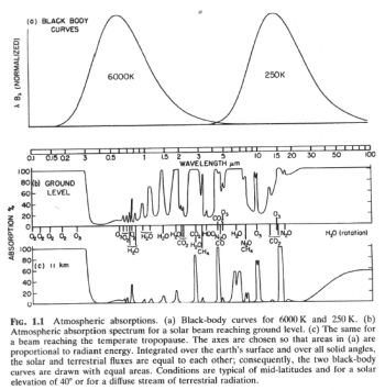
However, they have a mistake in a graph on p.4:

Kramm & Dlugi say:

..This figure also shows the atmospheric absorption spectrum for a solar beam reaching the ground level (b) and the same for a beam reaching the temperate tropopause (c) adopted from Goody and Yung [30]. Part (a) of Figure 5 completely differs from the original twin-peak diagram of Goody and Yung. We share the argument of Gerlich and Tscheuschner [2,4] that the original one is physically misleading..

I have the same argument about this one graph from Goody & Yung’s textbook. You can see my equivalent graph in 4th & 5th figures of The Sun and Max Planck Agree – Part Two.

There is nothing in the development of theory by Goody & Yung that depends on this graph. Kramm & Dlugi don’t demonstrate anything else in error from Goody & Yung. However, I’m sure that someone who wants to devote enough time to the subject will probably find another error in their book, or at least, an incautious statement that could imply that they have carelessly tossed away their knowledge of basic physics. This is left as an exercise for the interested reader..

To clarify the idea for readers – the energy emitted by the climate system to space is approximately equal to the energy absorbed from the sun by the climate system. This is not in dispute.

Kramm & Dlugi point out that one should be careful when attempting to plot equal areas on logarithmic graphs. Nice point.

Kepler & Milankovitch

Kramm & Dugli spend some time deriving the equations of planetary motion. These had been lost by climate science so it is good to see them recovered.

They also comment on Milankovitch’s theory in terms that are interesting:

Thus, on long-term scales of many thousands of years (expressed in kyr) we have to pay attention to Milankovitch’s [33] astronomical theory of climatic variations that ranks as the most important achievement in the theory of climate in the 20th century [10].

The theory definitely has a lot of mainstream support as being the explanation for the ice ages. However, as a comment to be developed one day when I understand enough to write about it, there isn’t one Milankovitch theory, there are many, and of necessity they contradict each other.

Interesting as well to suggest it as the most important achievement in the theory of climate last century – as the consequence of accepting Milankovitch’s theory is that climate is very sensitive to small peturbations in radiative changes in particular regions at particular times. In essence, the Milankovitch theory appears to rely on quite a high climate sensitivity.

Anyway, I’m not criticizing Kramm & Dugli or saying they are wrong. It’s just an interesting comment. And excellent that Kepler’s theories are no longer lost to the world of climate science.

Energy Conversion in the Atmosphere & at the Surface

The authors devote some time to this study (with no apparent differences to standard climate science) with the conclusion:

..Note that the local flux quantities like Q(θ, φ), H(θ, φ), G(θ, φ) and R_L↑(θ, φ) are required to calculate global averages of these fluxes, but not global averages of respective values of temperature and humidity.

An important point.

They also confirm – as noted in Kramm & Dlugi On Illuminating the Confusion of the Unclear – that the energy balance at the surface is affected by the energy radiated by the atmosphere. Just helping out the many blog writers and blog commenters – be sure to strike Kramm & Dlugi off your list of advocates of the imaginary second law of thermodynamics.

The Gulags for Everyone? – Climatology Loses Its Rational Basis

The authors cite this extract from the WMO website about the “greenhouse” effect:

In the atmosphere, not all radiation emitted by the Earth surface reaches the outer space. Part of it is reflected back to the Earth surface by the atmosphere (greenhouse effect) leading to a global average temperature of about 14°C well above –19°C which would have been felt without this effect.

This website statement is incorrect as the radiation emitted by the Earth’s surface is absorbed and re-emitted by the atmosphere – not reflected. This is a very basic error.

Kramm & Dlugi say:

Note that the argument that “part of it is reflected back to the Earth surface by the atmosphere” is completely irrational from a physical point of view. Such an argument also indicates that the discipline of climatology has lost its rational basis. Thus, the explanation of the WMO is rejected..

[Emphasis added]

Well, we could argue that if one person writing a website for one body writes one thing that is not technically correct then that whole discipline has lost its rational basis. We could.

Seems uncharitable to me. Although I have to confess that on occasion I am a little bit uncharitable. I wrote that Gerlich & Tscheuschner had lost their marbles, or were having a big laugh, with their many ridiculous and unfounded statements. We all have our off days.

I think if we want to uphold high standards of defendable technical accuracy we would say that the person that wrote this website and the person that reviewed this website are not technically sound as far as the specifics of radiative physics go. I’m hard pressed to think it is justified to cast stones at say Prof. Richard M Goody for this particular travesty. Or Prof. R. Lindzen. Or Prof. V. Ramanathan. Or Prof. F.W. Taylor. Otherwise it might be a bit like Stalin with the Gulag. Everyone and their mother gets tarred with the sins of the fellow down the road and 30 million people wind up digging rocks out of the ground in a very cold place..

But let’s stay on topic. If indeed there is one.

The Main Point

Now that we have found a graph in Goody that is wrong, a website that has a mistake and have rediscovered Kepler’s equations of motion, we turn to the main course.

Kramm & Dlugi turn to perhaps their main point, about the surface temperature of the earth with and without radiatively-active gases.

As a clarification for newcomers, average temperature has many problems. Due to the non-linearity of radiative physics, if we calculate the average radiation from the average temperature we will get a different answer compared with calculating the radiation from the temperature at each location/time and then taking the average.

For more on this basic topic see under the subheading How to Average in Why Global Mean Surface Temperature Should be Relegated, Or Mostly Ignored

First citing Lacis et al:

The difference between the nominal global mean surface temperature (TS = 288 K) and the global mean effective temperature (TE = 255 K) is a common measure of the terrestrial greenhouse effect (GT = TS – TE = 33 K).

The authors develop some maths, of which this is just a sample:

Using Eq. 3.8 and ignoring G(θ,φ) will lead to:

<T_s> = 2^3/2T_e/5 ≈ 144K (3.9)

for a non-rotating Earth in the absence of its atmosphere, if S = 1367 W/m² , α (Θ₀, θ, φ) = α_E = 0.30 and ε(θ, φ) = ε = 1 are assumed [2]

T_s = 153 K if α_E = 0.12 and T_s = 155 K if α_E = 0.07

It might surprise readers that these particular points are not something novel or in contradiction to the “greenhouse” effect. In fact, you can see similar points in two articles (at least) on this blog:

– In The Hoover Incident we had a look at what would happen to the climate if all the radiatively-active gases (= “greenhouse” gases) were removed from the atmosphere. Here is an extract:

..And depending on the ice sheet extent and whether any clouds still existed the value of outgoing radiation might be around 1.0 – 1.5 x 10¹⁷ W. This upper value would depend on the ice sheets not growing and all the clouds disappearing which seems impossible, but it’s just for illustration.

Remember that nothing in all this time can stop the emitted radiation from the surface making it to space. So the only changes in the energy balance can come from changes to the earth’s albedo (affecting absorbed solar radiation).

And given that when objects emit more energy than they absorb they cool down, the earth will certainly cool. The atmosphere cannot emit any radiation so any atmospheric changes will only change the distribution of energy around the climate system.

What would the temperature of the earth be? I have no idea..

Notice the heresy that without “greenhouse” gases we can’t say for sure what the surface temperature would be.. (It’s definitely going to be significantly lower though).

– In Atmospheric Radiation and the “Greenhouse” Effect – Part One:

..The average for 2009 [of outgoing longwave radiation] is 239 W/m². This average includes days, nights and weekends. The average can be converted to the total energy emitted from the climate system over a year like this:

Total energy radiated by the climate system into space in one year = 239 x number of seconds in a year x area of the earth in meters squared..

E_TOA= 3.8 x 10²⁴ J

The reason for calculating the total energy in 2009 is because many people have realized that there is a problem with average temperatures and imagine that this problem is carried over to average radiation. Not true. We can take average radiation and convert it into total energy with no problem..

[Emphasis added]

The point here is that the total emitted top of atmosphere radiation is much lower than the total surface emitted radiation. It can be calculated. In that article I haven’t actually attempted to do it accurately – it would require some work (spatial and temporal temperature across a year and the longwave emissivity of the surface around the globe) – it is a straightforward yet tedious calculation. (See note 2).

A note in passing that this difference between the top of atmosphere radiation and the surface radiation is also derided by the internet imaginary second law advocates as being a physical impossibility because it “creates energy”.

Now I am not in any way a “representative of climate science” despite the many claims to this effect, it’s just that the basics are.. the basics. And radiative transfer in the atmosphere is a technical yet simple subject which can be easily solved with the aid of some decent computing power. So I have no quarrel with anything of substance that I have so far read in textbooks or papers on radiative physics. Yet I appear to have stated similar points to Kramm & Dlugi.

Perhaps Kramm & Dlugi have not yet stated anything controversial on the inappropriately-named “greenhouse” effect.

They take issue with what I would call the “introduction to the greenhouse effect” where a simple comparison is drawn. This is where the “greenhouse” effect is highlighted as “effective temperature”.

It could more accurately be highlighted as “difference in average flux between surface and TOA” or “difference in total flux between surface and TOA”

Is it of consequence to anything in climate science if we agreed that the difference between the TOA radiation to space and the upward surface radiation is a better measure of the “greenhouse” effect?

Kramm & Dlugi comment on a paper by Ramanathan et al:

“At a surface temperature of 288 K the long-wave emission by the surface is about 390 W/m², whereas the outgoing long-wave radiation at the top of the atmosphere is only 236 W/m² (see Figure 2 [here presented as Figure 17]). Thus the intervening atmosphere causes a significant reduction in the long-wave emission to space. This reduction in the long-wave emission to space is referred to as the greenhouse effect”

As discussed before, applying the power law of Stefan and Boltzmann to a globally averaged temperature cannot be justified by physical and mathematical reasons.

Thus, the argument that at a surface temperature of 288 K the long-wave emission by the surface is about 390 W/m² is meaningless.

Just for interest here is how Ramanathan et al described their paper:

The two primary objectives of this review paper are (1) to describe the new scientific challenges posed by the trace gas climate problem and to summarize current strategies for meeting these challenges and (2) to make an assessment 0f the trace gas effects on troposphere-stratosphere temperature trends for the period covering the pre-industrial era to the present and for the next several decades. We will rely heavily on the numerous reports..

We could assume they don’t understand science basics, despite their many excellent papers demonstrating otherwise. Or we could assume that someone writing their 100th paper in the field of climate science doesn’t need to demonstrate that something called the “greenhouse” effect exists, or quantify it accurately in some specific way unless that is necessary for the specific purpose of the paper.

However, this is the genius of Kramm & Dlugi’s paper..

Dodging the Bullet

Casual readers of this paper (and people who rely on the statements of others about this paper) might think that they had demonstrated that the “greenhouse” effect doesn’t exist. They make a claim in their conclusion, of course, but they haven’t proven anything of the sort.

Instead they have written a paper explaining what everyone in climate science already knows.

So, to clarify matters, what is the emission of radiation from the top of atmosphere to space in one year?

E_TOA= 3.8 x 10²⁴ J

What is the emission of radiation from the surface in one year?

E_surface = ?

My questions to Kramm & Dlugi:

Is E_surface significantly greater than E_TOA ?

Obviously I believe Kramm & Dlugi will answer “Yes” to this question. This confirms the existence of the greenhouse effect, which they haven’t actually disputed except in their few words at the conclusion of their paper.

Hopefully, the authors will show up and confirm these important points.

Conclusion

The authors have shown us:

that a graph in the seminal Goody & Yung textbook is wrong
Kepler’s laws of planetary motion
that a website describes the “greenhouse” effect inaccurately
that without any “greenhouse” gases the effective albedo of the earth would be different
the average temperature of the earth’s surface can’t be used to calculate the average upward surface radiation

However, the important calculations of “radiative forcing” and various effects of increasing concentrations of radiatively-active gases are all done without using the “33K greenhouse effect”.

Without using the 33K “greenhouse” effect, we can derive all the equations of radiative transfer, solve them using the data for atmospheric temperature profiles, concentration of “greenhouse” gases, spectral line data from the HITRAN database and get:

the correct flux and spectral intensity at top of atmosphere
the correct flux and spectral intensity of downward radiation at the surface

We can also do this for changes in concentrations of various gases and find out the changes in top of atmosphere and downward surface flux. (Feedback and natural climate variations are the tricky part).

The discussions about average temperature are an amusing sideshow.

They are of no consequence for deriving the “greenhouse” effect or for determining the changes that might take place in the climate from increases or decreases in these gases.

Notes

Note 1: I didn’t check everything, so there could be mistakes. As the full article makes clear, not much need to check. I don’t endorse their last paragraph, as my conclusion – and article – makes clear.

Note 2: The calculation in that article for total annual global surface radiation doesn’t take into account surface emissivity. The value of ocean emissivity is incorrectly stated (see Emissivity of the Ocean). There are probably numerous other errors which I will fix one day if someone points them out.

Posted in Basic Science, Commentary | 162 Comments »

Kramm & Dlugi On Illuminating the Confusion of the Unclear

January 3, 2012 by scienceofdoom

Many people are confused about science basics when it comes to the inappropriately-named “greenhouse” effect.

This can be easily demonstrated in many blogs around the internet where commenters, and even blog owners, embrace multiple theories that contradict each other but are somehow against the “greenhouse” effect.

Recently a new paper: Scrutinizing the atmospheric greenhouse effect and its climatic impact by Gerhard Kramm & Ralph Dlugi was published in the journal Natural Science.

Because of their favorable comments about Gerlich & Tscheuschner and the fact that they are sort of against something called the “greenhouse” effect I thought it might be useful for many readers to find out what was actually in the paper and what Kramm & Dlugi actually do believe about the “greenhouse” effect.

Much of the comments on blogs about the “greenhouse” effect are centered around the idea that this effect cannot be true because it would somehow violate the second law of thermodynamics. If there was a scientific idea in Gerlich & Tscheuschner, this was probably the main one. Or at least the most celebrated.

So it might surprise readers who haven’t opened up this paper that the authors are thoroughly 100% with mainstream climate science (and heat transfer basics) on this topic.

It didn’t surprise me because before reading this paper I read another paper by Kramm – A case study on wintertime inversions in Interior Alaska with WRF, Mölders & Kramm, Atmospheric Research (2010).

This 2010 paper is very interesting and evaluates models vs observations of the temperature inversions that take place in polar climates (where the temperature at the ground in wintertime is cooler than the atmosphere above). Nothing revolutionary (as with 99.99% of papers) and so of course the model used includes a radiation scheme from CAM3 (=Community Atmospheric Model) that is well used in standard climate science modeling.

Here is an important equation from Kramm & Dlugi’s recent paper for the energy balance at the earth’s surface.

Lots of blogs “against the greenhouse effect” don’t believe this equation:

Figure 1

The highlighted term is the downward radiation from the atmosphere multiplied by the absorptivity of the earth’s surface (its ability to absorb the radiation). This downward radiation (DLR) has also become known as “back radiation”.

In simple terms, the energy balance of Kramm & Dlugi adds up the absorbed portions of the solar radiation and atmospheric longwave radiation and equates them to the emitted longwave radiation plus the latent and sensible heat.

So the temperature of the surface is determined by solar radiation and “back radiation” and both are treated equally. It is also determined of course by the latent and sensible heat flux. (And see note 1).

As so many people on blogs around the internet believe this idea violates the second law of thermodynamics I thought it would be helpful to these readers to let them know to put Kramm & Dlugi 2011 on their “wrong about the 2nd law” list.

Of course, many people “against the greenhouse thing” also – or alternatively – believe that “back radiation” is negligible. Yet Kramm & Dlugi reproduce the standard diagram from Trenberth, Fasullo & Kiehl (2009) and don’t make any claim about “back radiation” being different in value from this paper.

“Back radiation” is real, measurable and affects the temperature of the surface – clearly Kramm & Dlugi are AGW wolves in sheeps’ clothing!

I look forward to the forthcoming rebuttal by Gerlich & Tscheuschner.

In the followup article, Kramm & Dlugi On Dodging the “Greenhouse” Bullet, I will attempt to point out the actual items of consequence from their paper.

Further reading – Understanding Atmospheric Radiation and the “Greenhouse” Effect – Part One and New Theory Proves AGW Wrong!

Note 1 – The surface energy balance isn’t what ultimately determines the surface temperature. The actual inappropriately-named “greenhouse” effect is determined by:

the effective emission height to space of outgoing longwave radiation which is determined by the opacity of the atmosphere (for example, due to increases in CO2 or water vapor)
the temperature difference between the surface and the effective emission height which is determined by the lapse rate

Posted in Basic Science, Commentary | 242 Comments »

Measuring Climate Sensitivity – Part Three – Eddy Diffusivity

December 31, 2011 by scienceofdoom

In the last article we had a look at the depth of the “mixed ocean layer” (MLD) and its implications for the successful measurement of climate sensitivity (assuming such a parameter exists as a constant).

In Part One I created a Matlab model which reproduced the same problems as Spencer & Braswell (2008) had found. This model had one layer (an “ocean slab” model) to represent the MLD with a “noise” flux into the deeper ocean (and a radiative noise flux at top of atmosphere). Murphy & Forster claimed that longer time periods require an MLD of increased depth to “model” the extra heat flow into the deeper ocean over time:

Because heat slowly penetrates deeper into the ocean, an appropriate depth for heat capacity depends on the length of the period over which Eq. (1) is being applied (Watterson 2000; Held et al. 2010). For 80-yr global climate model runs, Gregory (2000) derived an optimum mixed layer depth of 150 m. Watterson (2000) found an initial global heat capacity equivalent to a mixed layer of 200 m and larger values for longer simulations.

This seems like it might make sense – if we wanted to keep a “zero dimensional model”. But it’s questionable whether the model retains any value with this “fudge”. So because heat actually moves from the mixed layer into the deeper ocean (rather than the mixed layer increasing in depth) I instead enhanced the model to create a heat flux from the MLD through a number of ocean layers with a parameter called the vertical eddy diffusivity to determine this heat flux.

So the model is now a 1D model with a parameterized approach to ocean convection.

Eddy Diffusivity

The concept here is the analogy of conductivity but when convection is instead the primary mover of heat.

Heat flow by conduction is governed by a material property called conductivity and by the temperature difference. Changes in temperature are governed by heat flow and by the heat capacity. The result is this equation for reference and interest – so don’t worry if you don’t understand it:

∂T / ∂t = α . ∂²T / ∂z² – the 1-d version (see note 1)

where T = temperature, t = time, α = thermal diffusivity and z = depth

What it says in almost plain English is that the change in temperature with respect to time is equal to the thermal diffusivity times the change in gradient of temperature with depth. Don’t worry if that’s not clear (and there is a explanation of the simple steps required to calculate this in note 1).

Now the thermal diffusivity, α:

α = k/c_pρ, where k = conductivity, c_p = heat capacity and ρ = density

So, an important bit to understand..

if the conductivity is high and the heat capacity is low then temperature can change quickly
if the conductivity is high and the heat capacity is high then it slows down temperature change, and
if the conductivity is low and the heat capacity is high then temperature takes much longer to change

Many researchers have attempted to measure an average value for eddy diffusivity in the ocean (and in lakes). The concept here, an explained in Part Two, is that turbulent motions of the ocean move heat much more effectively than conduction. The value can’t be calculated from first principles because that would mean solving the problem of turbulence, which is one of the toughest problems in physics. Instead it has to be estimated from measurements.

There is an inherent problem with eddy diffusivity for vertical heat transfer that we will come back to shortly.

There is also a minor problem of notation that is “solved” here by changing the notation. Usually conductivity is written as “k”. However, most papers on eddy diffusivity write diffusivity as “k”, sometimes “K”, sometimes “κ” (Greek ‘kappa’) – creating potential confusion so I revert back to “α”. And to make it clear that it is the convective value rather than the conductive value, I use α_eddy. And for the equivalent parameter to conductivity, k_eddy.

k_eddy = α_eddyc_pρ

because c_p= 4200 J/K.kg and ρ ≈ 1000 kg/m³:

k_eddy =4.2 x 10⁶ α_eddy – it’s useful to be able to see what the diffusivity means in terms of an equivalent “conductivity” type parameter

Measurements of Eddy Diffusivity

Oeschger et al (1975):

α is an apparent global eddy diffusion coefficient which helps to reproduce an average transport phenomenon consisting of a series of distinct and overlapping mechanisms.

Oeschger and his co-workers studied the problem via the diffusion into the ocean of ¹⁴C from nuclear weapons testing.

The range they calculated for α_eddy = 1 x 10^-4 – 1.8 x 10^-4 m²/s.

This equates to k_eddy = 420 – 760 W/m.K, and by comparison, the conductivity of still water, k = 0.6 W/m.K – making convection around 1,000 times more effective at moving heat vertically through the ocean.

Broecker et al (1980) took a similar approach to estimating this value and commented:

We do not mean to imply that the process of vertical eddy mixing actually occurs within the body of the main oceanic thermocline. Indeed, the values we require are an order of magnitude greater than those permitted by conventional oceanographic wisdom (see Garrett, 1979, for summary).

The vertical eddy coefficients used here should rather be thought of as parameters that take into account all the processes that transfer tracers across density horizons. In addition to vertical mixing by eddies, these include mixing induced by sediment friction at the ocean margins and mixing along the surface in the regions where density horizons outcrop.

Their calculation, like Oeschger’s, used a simple model with the observed values plugged in to estimate the parameter:

Anyone familiar with the water mass structure and ventilation dynamics of the ocean will quickly realize that the box-diffusion model is by no means a realistic representation. No simple modification to the model will substantially improve the situation.

To do so we must take a giant step in complexity to a new generation of models that attempt to account for the actual geometry of ventilation of the sea. We are as yet not in a position to do this in a serious way. At least a decade will pass before a realistic ocean model can be developed.

The values they calculated for eddy diffusivity were broken up into different regions:

α_eddy(equatorial) = 3.5 x 10^-5 m²/s
α_eddy(temperate) = 2.0 x 10^-4 m²/s
α_eddy(polar) = 3.0 x 10^-4 m²/s

We will use these values from Broecker to see what happens to the measurement problems of climate sensitivity when used in my simple model.

These two papers were cited by Hansen et al in their 1985 paper with the values for vertical eddy diffusivity used to develop the value of the “effective mixed depth” of the ocean.

In reviewing these papers and searching for more recent work in the field, I tapped into a rich vein of research that will be the subject of another day.

First, Ledwell et al (1998) who measured eddy diffusivity via SF₆ that they injected into the ocean:

The diapycnal eddy diffusivity K estimated for the first 6 months was 0.12 ± 0.02 x10^-4 m²/s, while for the subsequent 24 months it was 0.17 ± 0.02 x10^-4 m²/s.

[Note: units changed from cm²/s into m²/s for consistency]

It is worth reading their comment on this aspect of ocean dynamics. (Note that isopycnal = contact density surfaces and diapycnal = across isopycnal):

The circulation of the ocean is severely constrained by density stratification. A water parcel cannot move from one surface of constant potential density to another without changing its salinity or its potential temperature. There are virtually no sources of heat outside the sunlit zone and away from the bottom where heat diffuses from the lithosphere, except for the interesting hydrothermal vents in special regions. The sources of salinity changes are similarly confined to the boundaries of the ocean. If water in the interior is to change potential density at all, it must be by mixing across density surfaces (diapycnal mixing) or by stirring and mixing of water of different potential temperature and salinity along isopycnal surfaces (isopycnal mixing).

Most inferences of dispersion parameters have been made from observations of the large-scale fields or from measurements of dissipation rates at very small scales. Unambiguously direct measurements of the mixing have been rare. Because of the stratification of the ocean, isopycnal mixing involves very different processes than diapycnal mixing, extending to much greater length scales. A direct approach to the study of both isopycnal and diapycnal mixing is to release a tracer and measure its subsequent dispersal. Such an experiment, lasting 30 months and involving more than 10⁵ km² of ocean, is the subject of this paper.

From Jayne (2009):

For example, the Community Climate Simulation Model (CCSM) ocean component model uses a form similar to Eq. (1), but with an upper-ocean value of 0.1 x 10^-4 m²/s and a deep-ocean value of 1.0 x 10^-4 m²/s, with the transition depth at 1000 m.

However, there is no observational evidence to suggest that the mixing in the ocean is horizontally uniform, and indeed there is significant evidence that it is heterogeneous with spatial variations of several orders of magnitude in its intensity (Polzin et al. 1997; Ganachaud 2003).

More on eddy diffusivity measurements in another article – the parameter has a significant impact on modeling of the ocean in GCMs and there is a lot of current research into this subject.

Eddy Diffusivity and Buoyancy Gradient

Sarmiento et al (1976) measured isotopes near the ocean floor:

Two naturally occurring isotopes can be applied to the determination of the rate of vertical turbulent mixing in the deep sea: ²²²Rn (half-life 3.824 days) and ²²⁸Ra (half-life 5.75 years). In this paper we discuss the results from fourteen ²²²Rn and two ²²⁸Ra profiles obtained as part of the GEOSECS program.

From these results we conclude that the most important factor influencing the vertical eddy diffusivity is the buoyancy gradient [(g/p)(∂ρ_pot/∂z)]. The vertical diffusivity shows an inverse proportionality to the buoyancy gradient.

Their paper is very much about the measurements and calculations of the deeper ocean, but is relevant for anywhere in the ocean, and helps explain why the different values for different regions were obtained by Broecker that we saw earlier. (Prof. Wallace S. Broecker was a co-author on this paper as well, and has authored/co-authored 100’s of papers on the ocean).

What is the buoyancy gradient and why does it matter?

Cold fluids sink and hot fluids rise. This is because cold substances contract and so are more dense. So in general, in the ocean, the colder water is below and the warmer water above. Probably everyone knows this.

The buoyancy gradient is a measure of how strong this effect is. The change in density with depth determines how resistant the ocean is to being overturned. If the ocean was totally stable no heat would ever penetrate below the mixed layer. But it does. And if the ocean was totally stable then the measurements of ¹⁴C from nuclear testing would be zero below the mixed layer.

But it is not surprising that the more stable the ocean is due to the buoyancy gradient the less heat diffuses down by turbulent motion.

And this is why the estimates by Broecker shown earlier have a much lower value of diffusivity for the tropics than for the poles. In general the poles are where deep convection takes place – lots of cold water sinks, mixing the ocean – and the tropics are where much weaker upwelling takes place – because the ocean surface is strongly heated. This is part of the large scale motion of the ocean, known as the thermohaline circulation. More on this another day.

Now water is largely incompressible which means that the density gradient is only determined by temperature and salinity. This creates the problem that eddy diffusivity is a value which is not only parameterized, but also dependent on the vertical temperature difference in the ocean.

Heat flow also depends on temperature difference, but with the opposite relationship. This is not something to untangle today. Today we will just see what happens to our simple model when we use the best estimates of vertical eddy diffusivity.

Modeling, Non-Linearity and Climate Sensitivity Measurement Problems

Murphy & Forster agreed in part with Spencer & Braswell about the variation in radiative noise from CERES measurements. I quote at length, because the Murphy & Forster paper is not freely available:

For the parameter N, SB08 use a random daily shortwave flux scaled so that the standard deviation of monthly averages of outgoing radiation (N – λT) is 1.3 W/m².

They base this on the standard deviation of CERES shortwave data between March 2000 and December 2005 for the oceans between 20 °Nand 20 °S.

We have analyzed the same dataset and find that, after the seasonal cycle and slow changes in forcing are removed, the standard deviation of monthly means of the shortwave radiation is 1.24 W/m², close to the 1.3 W/m² specified by SB08. However, longwave (infrared) radiation changes the energy budget just as effectively from the earth as shortwave radiation (reflected sunlight). Cloud systems that might induce random fluctuations in reflected sunlight also change outgoing longwave radiation. In addition, the feedback parameter λ is due to both longwave and shortwave radiation.

Modeled total outgoing radiation should therefore be compared with the observed sum of longwave and shortwave outgoing radiation, not just the shortwave component. The standard deviation of the sum of longwave and shortwave radiation in the same CERES dataset is 0.94 W/m². Even this is an upper limit, since imperfect spatial sampling and instrument noise contribute to the standard deviation.

[Note I change their α (climate feedback) to λ for consistency with previous articles].

And they continue:

We therefore use 0.94 W/m² as an upper limit to the standard deviation of outgoing radiation over the tropical oceans. For comparison, the standard deviation of the global CERES outgoing radiation is about 0.55 W/m².

All of these points seem valid (however, I am still in the process of examining CERES data, and can’t comment on their actual values of standard deviation. Apart from the minor challenge of extracting the data from the netCDF format there is a lot to examine. A lot of data and a lot of issues surrounding data quality).

However, it raised an interesting idea about non-linearity. Readers who remember on Part One will know that as radiative noise increases and ocean MLD decreases the measurement problem gets worse. And as the radiative noise decreases and ocean MLD increases the measurement problem goes away.

If we average global radiative noise and global MLD, plug these values into a zero-dimensional model and get minimal measurement problem what does this mean?

Due to non-linearity, it tells us nothing.

Averaging the inputs, applying them to a global model (i.e., a zero-dimensional model) and calculating λ_est (from the regression) gets very different results from applying the inputs separately to each region, averaging the results and calculating λ_est

I tested this with a simple model – created two regions, one 10% of the surface area, the other 90%. In the larger region the MLD was 200m and the radiative noise was zero; and in the smaller region the MLD was 20m and the (standard deviation of) radiative noise was varied from 0 – 2. The temperature and radiative flux were converted into an area weighted time series and the regression produced large deviations from the real value of λ.

A similar run on a global model with an MLD of 180m and radiative noise of 0-0.2 shows an accurate assessment of λ.

This is to be expected of course.

So with this in mind I tested the new 1D model with different values of ocean depth eddy diffusivity, radiative noise, and an AR(1) model for the radiative noise. I used values for the tropical region as this is clearly the area most likely to upset the measurement – shallow MLD, higher radiative noise and weaker eddy diffusivity.

As best as I could determine from de Boyer Montegut’s paper, the average MLD for the 20°N – 20°S region is approximately 30m.

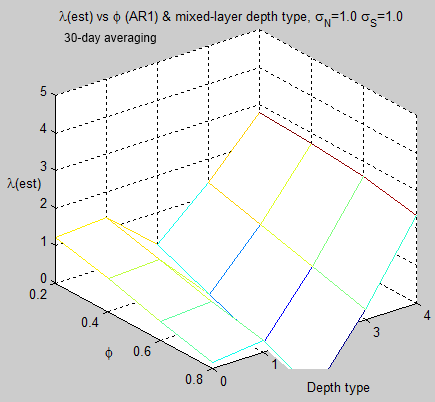
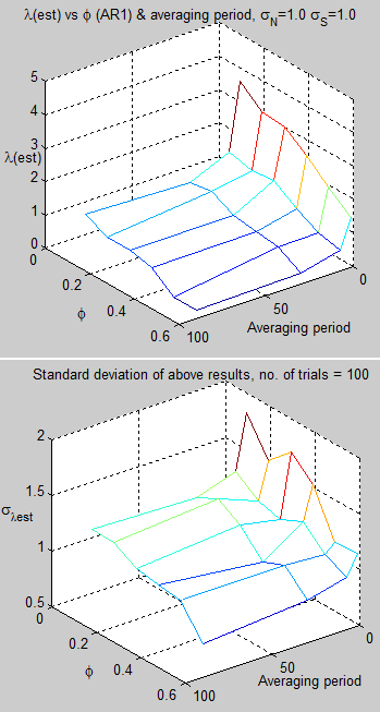
Here are the results using Oeschger’s value of eddy diffusivity for the tropics and the tropical value of radiative noise from MF2010 – varying ocean depth around 30m and the value of the AR(1) model for radiative noise:

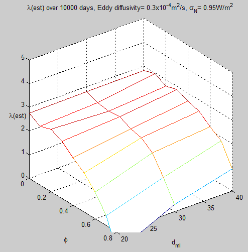
Figure 1

For reference, as it’s hard to read off the graph, the value at 30m and φ=0.5 is λ_est = 2.3.

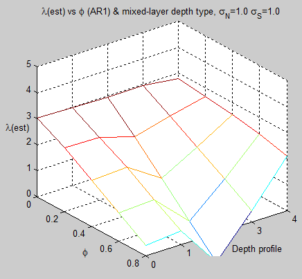
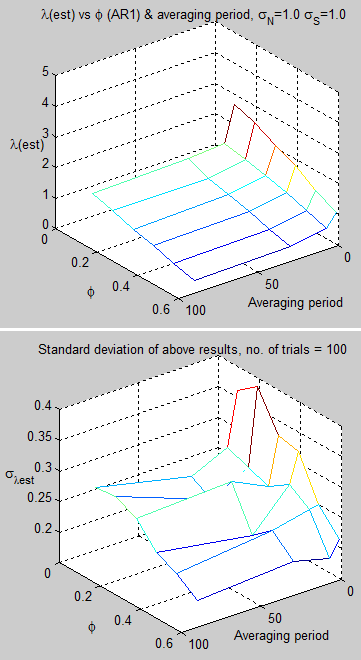
Using the current CCSM value of eddy diffusivity for the upper ocean:

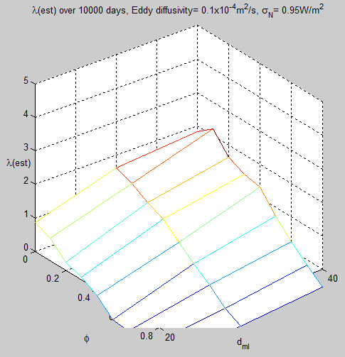
Figure 2

For reference, the value at 30m and φ=0.5 is λ_est = 0.2. (Compared with the real value of 3.0)

Note that these values are only for one region, not for the whole globe.

Another important point is that I have used the radiative noise value as the standard deviation of daily radiative noise. I have started to dig into CERES data to see whether such a value can be calculated, and also what typical value of autoregressive parameter should be used (and what kind of ARMA model), but this might take some time.

Yet smaller values of eddy diffusivity are possible for smaller regions, according to Jochum (2009). This would likely cause the problems of estimating climate sensitivity to become worse.

Simple Models

Murphy & Forster comment:

Although highly simplified, a single box model of the earth has some pedagogic value. One must remember that the heat capacity c and feedback parameter λ are not really constants, since heat penetrates more deeply into the ocean on long time scales and there are fast and slow climate feedbacks (Knutti et al. 2008).

It is tempting to add a few more boxes to account for land, ocean, different latitudes, and so forth. Adding more boxes to an energy balancemodel can be problematic because one must ensure that the boxes are connected in a physically consistent way. A good option is to instead consider a global climate model that has many boxes connected in a physically consistent manner.

The point being that no one believes a slab model of the ocean to be a model that gives really useful results. Spencer & Braswell likewise don’t believe that the slab model is in any way an accurate model of the climate.

They used such a model just to demonstrate a possible problem. Murphy & Forster’s criticism doesn’t seem to have solved the problem of “can we measure climate sensitivity?”

Or at least, it appears easy to show that slightly different enhancements of the simple model demonstrate continued problems in measuring climate sensitivity – due to the impact of radiative noise in the climate system.

Conclusion

I have produced a simple model and apparently demonstrated continued climate sensitivity measurement problems. This is in contrast to Murphy & Forster who took a different approach and found that the problem went away. However, my model has a more realistic approach to moving heat from the mixed layer into the ocean depths than theirs.

My model does have the drawback that the massive army of Science of Doom model testers and quality control champions are all away on their Xmas break. So the model might be incorrectly coded.

It’s also likely that someone else can come along and take a slightly enhanced version of this model and make the problem vanish.

I have used values for MLD and eddy diffusivity that seem to represent real-world values but I have no idea as to the correct values for standard deviation and auto-correlation of daily radiative noise (or appropriate ARMA model). These values have a big impact on the climate sensitivity measurement problem for reasons explained in Part One.

A useful approach to determining the effect of radiative noise on climate sensitivity measurement might be to use a coupled atmosphere-ocean GCM with a known climate sensitivity and an innovative way of removing radiative noise. These kind of experiments are done all the time to isolate one effect or one parameter.

Perhaps someone has already done this specific test?

I see other potential problems in measuring climate sensitivity. Here is one obvious problem – as the temperature of the mixed layer increases with continued increases in radiative forcing the buoyancy gradient increases and the eddy diffusivity reduces. We can calculate radiative forcing due to “greenhouse” gases quite accurately and therefore remove it from the regression analysis (see Spencer & Braswell 2008 for more on this). But we can’t calculate the change in eddy diffusivity and heat loss to the deeper ocean. This adds another “correlated” term that seems impossible to disentangle from the climate sensitivity calculation.

An alternative way of looking at this is that climate sensitivity might not be a constant – as already noted in Part One.

Articles in this Series

Measuring Climate Sensitivity – Part One

Measuring Climate Sensitivity – Part Two – Mixed Layer Depths

References

Potential Biases in Feedback Diagnosis from Observational Data: A Simple Model Demonstration, Spencer & Braswell, Journal of Climate (2008) – FREE

On the accuracy of deriving climate feedback parameters from correlations between surface temperature and outgoing radiation, Murphy & Forster, Journal of Climate (2010)

A box diffusion model to study the carbon dioxide exchange in nature, Oeschger et al, Tellus (1975)

Modeling the carbon system, Broecker et al, Radiocarbon (1980) – FREE

Climate response times: dependence on climate sensitivity and ocean mixing, Hansen et al, Science (1985)

The study of mixing in the ocean: A brief history, MC Gregg, Oceanography (1991) – FREE

Spatial Variability of Turbulent Mixing in the Abyssal Ocean, Polzin et al, Science (1997) – FREE

The Impact of Abyssal Mixing Parameterizations in an Ocean General Circulation Model, Steven R. Jayne, Journal of Physical Oceanography (2009)

The relationship between vertical eddy diffusion and buoyancy gradient in the deep sea, Sarmiento et al, Earth & Planetary Science Letters (1976)

Mixing of a tracer in the pycnocline, Ledwell et al, JGR (1998)

Impact of latitudinal variations in vertical diffusivity on climate simulations, Jochum, JGR (2009) – FREE

Mixed layer depth over the global ocean: An examination of profile data and a profile-based climatology, de Boyer Montegut et al, JGR (2004)

Notes

Note 1: The 1D version is really:

∂T / ∂t = ∂/∂z (α.∂T/∂z)

due to the fact that α can be a function of z (and definitely is in the case of the ocean).

Although this looks tricky – and it is tricky to find analytical solutions – solving the 1D version numerically is very straightforward and anyone can do it.

In plain English is looks something like:

– Heat flow into cell X = temperature difference between cell X and cell X-1

– Heat flow out of cell X = temperature difference between cell X and cell X+1

– Change in temperature = (Heat flow into cell X – Heat flow out of cell X) x time / heat capacity

Note 2: I am in the process of examining CERES data. Apart from the challenge of extracting the data from the netCDF format there is a lot to examine. A lot of data and a lot of issues surrounding data quality.

Posted in Measurement, Ocean Physics | 1 Comment »

Measuring Climate Sensitivity – Part Two – Mixed Layer Depths

December 23, 2011 by scienceofdoom

In Measuring Climate Sensitivity – Part One we saw that there can be potential problems in attempting to measure the parameter called “climate sensitivity”.

Using a simple model Spencer & Braswell (2008) had demonstrated that even when the value of “climate sensitivity” is constant and known, measurement of it can be obscured for a number of reasons.

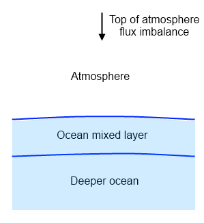
The simple model was a “slab model” of the ocean with a top of atmosphere imbalance in radiation.

Murphy & Forster (2010) criticized Spencer & Braswell for a few reasons including the value chosen for the depth of this ocean mixed layer. As the mixed layer depth increases the climate sensitivity measurement problems are greatly reduced.

First, we will consider the mixed layer in the context of that simple model. Then we will consider what it means in real life.

The Simple Model of Climate Sensitivity

The simple model used by Spencer & Braswell has a “mixed ocean layer” of depth 50m.

Figure 1

In the model the mixed layer is where all of the imbalance in top of atmosphere radiation gets absorbed.

The idea in the simple model is that the energy absorbed from the top of atmosphere gets mixed into the top layer of the ocean very quickly. In reality, as we will see, there isn’t such a thing as one layer but it is a handy approximation.

Murphy & Forster commented:

For the heat capacity parameter c, SB08 use the heat capacity of a 50-m ocean mixed layer. This is too shallow to be realistic.

Because heat slowly penetrates deeper into the ocean, an appropriate depth for heat capacity depends on the length of the period over which Eq. (1) is being applied (Watterson 2000; Held et al. 2010).

For 80-yr global climate model runs, Gregory (2000) derived an optimum mixed layer depth of 150 m. Watterson (2000) found an initial global heat capacity equivalent to a mixed layer of 200 m and larger values for longer simulations.

Held et al. (2010) found an initial time constant τ = c/α of about four yr in the Geophysical Fluid Dynamics Laboratory global climate model. Schwartz (2007) used historical data to estimate a globally averaged mixed layer depth of 150 m, or 106 m if the earth were only ocean.

The idea is an attempt to keep the simplicity of one mixed layer for the model, but increase the depth of this mixed layer for longer time periods.

There is always a point where models – simplified versions of the real world – start to break down. This might be the case here.

The initial model was of a mixed layer of ocean, all at the same temperature because the layer is well-mixed – and with some random movement of heat between this mixed layer and the ocean depths. In a more realistic scenario, more heat flows into the deeper ocean as the length of time increases.

What Murphy & Forster are proposing is to keep the simple model and “account” for the ever increasing heat flow into the deeper ocean by using a depth of the mixed layer that is dependent on the time period.

If we do this perhaps the model will work, perhaps it won’t. By “work” we mean provide results that tell us something useful about the real world.

So I thought I would introduce some more realism (complexity) into the model and see what happened. This involves a bit of a journey.

Real Life Ocean Mixed Layer

Water is a very bad conductor of heat – as are plastic and other insulators. Good conductors of heat include metals.

However, in the ocean and the atmosphere conduction is not the primary heat transfer mechanism. It isn’t even significant. Instead, in the ocean it is convection – the bulk movement of fluids – that moves heat. Think of it like this – if you move a “parcel” of water, the heat in that parcel moves with it.

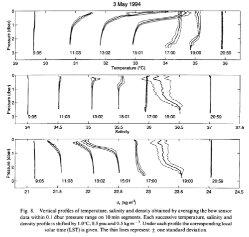
Let’s take a look at the temperature profile at the top of the ocean. Here the first graph shows temperature:

Soloviev & Lukas (1997)

Figure 2

Note that the successive plots are not at higher and higher temperatures – they are just artificially separated to make the results easier to see. During the afternoon the sun heats the top of the ocean. As a result we get a temperature gradient where the surface is hotter than a few meters down. At night and early morning the temperature gradient disappears. (No temperature gradient means that the water is all at the same temperature)

Why is this?

Once the sun sets the ocean surface cools rapidly via radiation and convection to the atmosphere. The result is colder water, which is heavier. Heavier water sinks, so the ocean gets mixed. This same effect takes place on a larger scale for seasonal changes in temperature.

And the top of the ocean is also well mixed due to being stirred by the wind.

A comment from de Boyer Montegut and his coauthors (2004):

A striking and nearly universal feature of the open ocean is the surface mixed layer within which salinity, temperature, and density are almost vertically uniform. This oceanic mixed layer is the manifestation of the vigorous turbulent mixing processes which are active in the upper ocean.

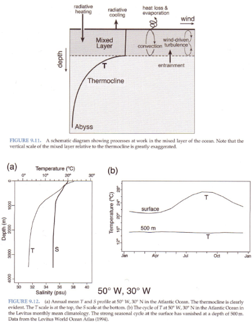
Here is a summary graphic from the excellent Marshall & Plumb:

From Marshall & Plumb (2008)

Figure 3

There’s more on this subject in Does Back-Radiation “Heat” the Ocean? – Part Three.

How Deep is the Ocean Mixed Layer?

This is not a simple question. Partly it is a measurement problem, and partly there isn’t a sharp demarcation between the ocean mixed layer and the deeper ocean. Various researchers have made an effort to map it out.

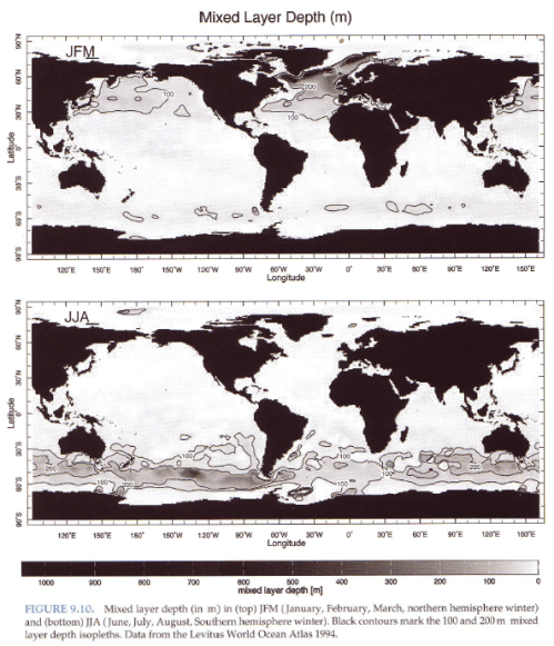
Here is a global overview, again from Marshall & Plumb:

Figure 4

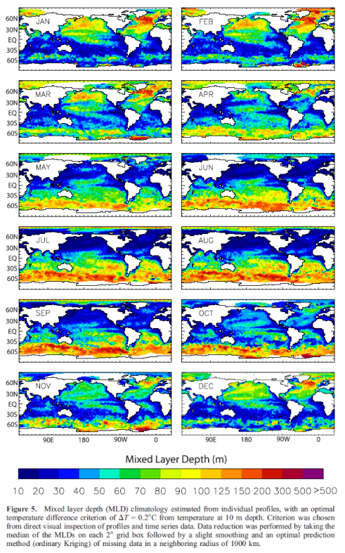
You can see that the deeper mixed layers occur in the higher latitudes.

Comment from de Boyer Montegut:

The main temporal variabilities of the MLD [mixed layer depth] are directly linked to the many processes occurring in the mixed layer (surface forcing, lateral advection, internal waves, etc), ranging from diurnal [Brainerd and Gregg, 1995] to interannual variability, including seasonal and intraseasonal variability [e.g., Kara et al., 2003a; McCreary et al., 2001]. The spatial variability of the MLD is also very large.

The MLD can be less than 20 m in the summer hemisphere, while reaching more than 500 m in the winter hemisphere in subpolar latitudes [Monterey and Levitus, 1997].

Here is a more complete map by month. Readers probably have many questions about methodology and I recommend reading the free paper:

From de Boyer Montegut et al (2004)

Figure 5 – Click for a larger image

Seeing this map definitely had me wondering about the challenge of measuring climate sensitivity. Spencer & Braswell had used 50m MLD to identify some climate sensitivity measurement problems. Murphy & Forster had reproduced their results with a much deeper MLD to demonstrate that the problems went away.

But what happens if instead we retest the basic model using the actual MLD which varies significantly by month and by latitude?

So instead of “one slab of ocean” at MLD = choose your value, we break up the globe into regions, have different values in each region each month and see what happens to climate sensitivity problems.

By the way, I also attempted to calculate the global annual (area weighted) average of MLD from the maps above, by eye. I also emailed the author of the paper to get some measurement details but no response.

My estimate of the data in this paper was a global annual area weighted average of 62 meters.

Trying Simple Models with Varying MLD

I updated the Matlab program from Measuring Climate Sensitivity – Part One. The globe is now broken up into 30º latitude bands, with the potential for a different value of mixed layer depth for each month of the year.

I created a number of different profiles:

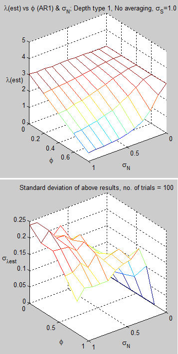
Depth Type 0 – constant with month and latitude, as in the original article

Type 1 – using the values from de Boyer’s paper, as best as can be estimated from looking at the monthly maps.

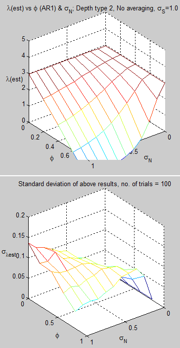
Type 2 – no change each month, with scaling of 60ºN-90ºN = 100x the value for 0ºN – 30ºN, and 30ºN – 60ºN = 10x the value for 0ºN – 30ºN – similarly for the southern hemisphere.

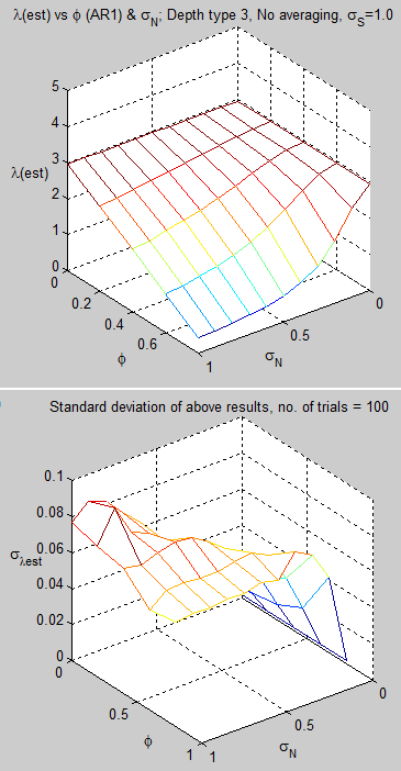
Type 3 – alternating each month between Type 2 and its inverse, i.e., scaling of 0ºN – 30ºN = 100x the value for 60ºN-90ºN and 30ºN – 60ºN = 10x the value for 60ºN-90ºN.

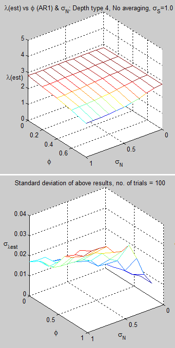
Type 4 – no variation by latitude, but month 1 = 1000x month 4, month 2 = 100x month 4, month 3 = 10x month 4, repeating 3 times per year.

In each case the global annual (area weighted) average = 62m.

Essentially types 2-4 are aimed at creating extreme situations.

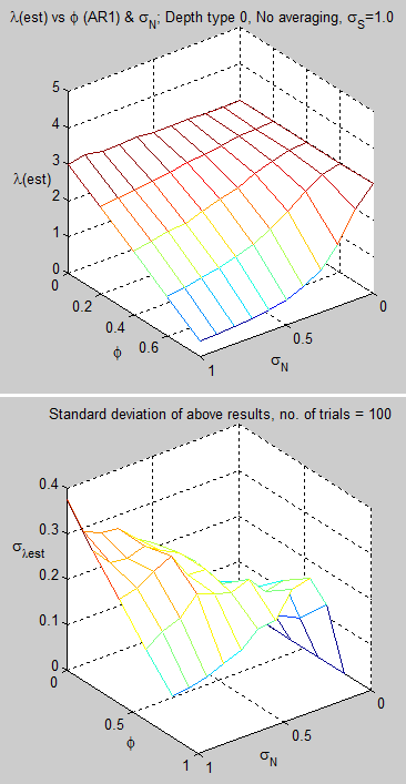
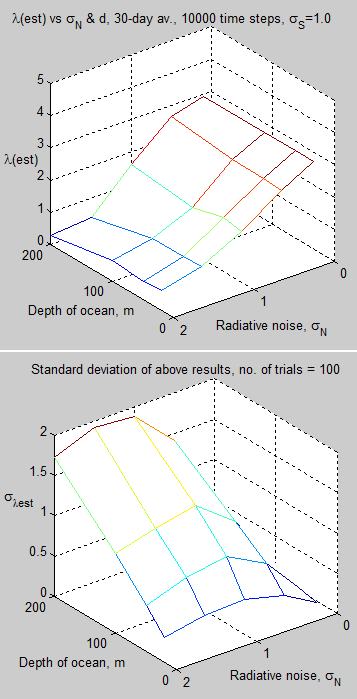
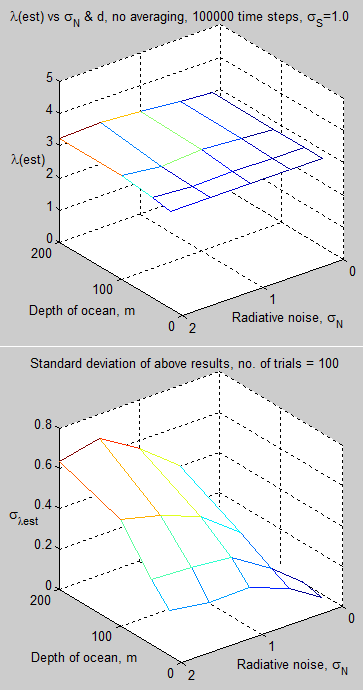
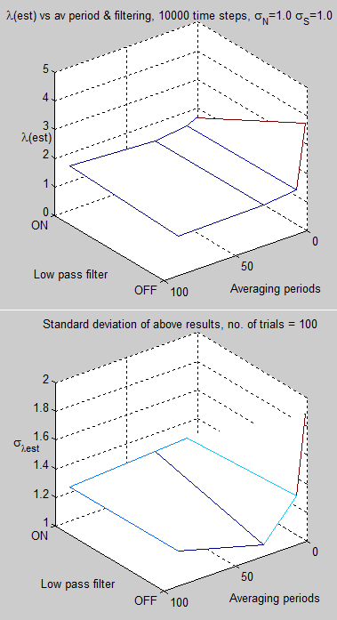
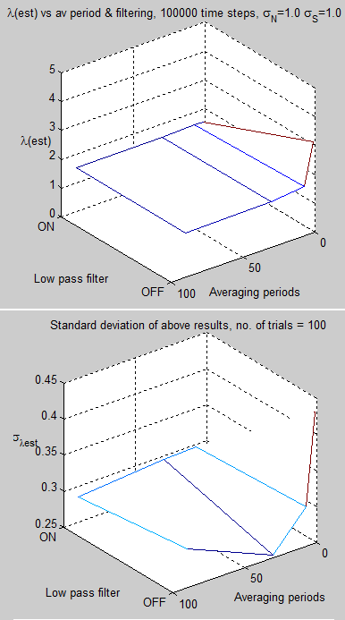
Here are some results (review the original article for some of the notation), recalling that the actual climate sensitivity, λ = 3.0:

Figure 6

Figure 7 – as figure 6 without 30-day averaging

Figure 8

Figure 9

Figure 10

Figure 11

Figure 12

What’s the message from these results?

In essence, type 0 (the original) and type 1 (using actual MLDs vs latitude and month from de Boyer’s paper) are quite similar – but not exactly the same.

However, if we start varying the MLD by latitude and month in a more extreme way the results come out very differently – even though the global average MLD is the same in each case.

This demonstrates that the temporal and area variation of MLD can have a significant effect and modeling the ocean as one slab – for the purposes of this enterprise – may be risky.

Non-Linearity

We haven’t considered the effect of non-linearity in these simple models. That is, what about interactions between different regions and months. If we created a yet more complex model where heat flowed between regions dependent on the relative depths of the mixed layers what would we find?

Losing the Plot?

Now, in case anyone has lost the plot by this stage – and it’s possible that I have – don’t get confused into thinking that we are evaluating GCM’s and gosh aren’t they simplistic.. No, GCM’s have very sophisticated modeling.

What we have been doing is tracing a path that started with a paper by Spencer & Braswell. This paper used a very simple model to show that with some random daily fluctuations in top of atmosphere radiative flux, perhaps due to clouds, the measurement of climate sensitivity doesn’t match the actual climate sensitivity.

We can do this in a model – prescribe a value and then test whether we can measure it. This is where this simple model came in. It isn’t a GCM.

However, Murphy & Forster came along and said if you use a deeper mixed ocean layer (which they claim is justified) then the measurement of climate sensitivity does more or less match the actual climate sensitivity (they also had comment on the values chosen for radiative flux anomalies, a subject for another day).

What struck me was that the test model needs some significant improvement to be able to assess whether or not climate sensitivity can be measured. And this is with the caveat – if climate sensitivity is a constant.

The Next Phase – More Realistic Ocean Model

As Murphy & Forster have pointed out, the longer the time period, the more heat is “injected” into the deeper ocean from the mixed layer.

So a better model would capture this better than just creating a deeper mixed layer for a longer time. Modeling true global ocean convection is an impossible task.

As a recap, conducted heat flow:

q” = k.ΔT/d

where q” = heat flow per unit area, k = conductivity, ΔT = temperature difference, and d = depth of layer

Take a look at Heat Transfer Basics – Part Zero for more on these basics.

For water, k = 0.6 W/m².K. So, as an example, if we have a 10ºC temperature difference across 1 km depth of water, q” = 0.006 W/m². This is tiny. Heat flow via conduction is insignificant. Convection is what moves heat in the ocean.

Many researchers have measured and estimated vertical heat flow in the ocean to come up with a value for vertical eddy diffusivity. This allows us to make some rough estimates of vertical heat flow via convection.

In the next version of the Matlab program (“in press”) the ocean is modeled with different eddy diffusivities below the mixed ocean layer to see what happens to the measurement of climate sensitivity. So far, the model comes up with wildly varying results when the eddy diffusivity is low, i.e., heat cannot easily move into the ocean depths. And it comes up with normal results when the eddy diffusivity is high, i.e., heat moves relatively quickly into the ocean depths.

Due to shortness of time, this problem has not yet been resolved. More in due course.

This article is already long enough, so the next part will cover the estimated values for eddy diffusivity because it’s an interesting subject

Conclusion

Regular readers of this blog understand that navigating to any kind of conclusion takes some time on my part. And that’s when the subject is well understood. I’m finding that the signposts on the journey to measuring climate sensitivity are confusing and hard to read.

And that said, this article hasn’t shed any more light on the measurement of climate sensitivity. Instead, we have reviewed more ways in which measurements of it might be wrong. But not conclusively.

Next up we will take a detour into eddy diffusivity, hoping in the meantime that the Matlab model problems can be resolved. Finally a more accurate model incorporating eddy diffusivity to model vertical heat flow in the ocean will show us whether or not climate sensitivity can be accurately measured.

Possibly.

Articles in this Series

Measuring Climate Sensitivity – Part One

Measuring Climate Sensitivity – Part Three – Eddy Diffusivity

References

Potential Biases in Feedback Diagnosis from Observational Data: A Simple Model Demonstration, Spencer & Braswell, Journal of Climate (2008)

On the accuracy of deriving climate feedback parameters from correlations between surface temperature and outgoing radiation, Murphy & Forster, Journal of Climate (2010)

Observation of large diurnal warming events in the near-surface layer of the western equatorial Pacific warm pool, Soloviev & Lukas, Deep Sea Research Part I: Oceanographic Research Papers (1997)

Atmosphere, Ocean and Climate Dynamics: An Introductory Text, Marshall & Plumb, Elsevier Academic Press (2008)

Mixed layer depth over the global ocean: An examination of profile data and a profile-based climatology, de Boyer Montegut et al, JGR (2004)

Posted in Measurement, Ocean Physics | 26 Comments »

The Creation of Time

November 17, 2011 by scienceofdoom

We all would like this machine that creates time.

In the context of Science of Doom all my time has been diverted into work-related activities and I’m not sure when this will ease up.

Unless someone hands me this machine, and for a price well below market worth, I am not sure when my next post will take place.

I have lots of ideas, but like to do research and gain understanding before writing articles.

Normal service will eventually be resumed.

Posted in Basic Science | 18 Comments »

Measuring Climate Sensitivity – Part One

September 22, 2011 by scienceofdoom

I don’t think this is a simple topic.

The essence of the problem is this:

Can we measure the top of atmosphere (TOA) radiative changes and the surface temperature changes and derive the “climate sensivity” from the relationship between the two parameters?

First, what do we mean by “climate sensitivity”?

In simple terms this parameter should tell us how much more radiation (“flux”) escapes to space for each 1°C increase in surface temperature.

Climate Sensitivity Is All About Feedback

Climate sensitivity is all about trying to discover whether the climate system has positive or negative feedback.

If the average surface temperature of the earth increased by 1°C and the radiation to space consequently increased by 3.3 W/m², this would be approximately “zero feedback”.

Why is this zero feedback?

If somehow the average temperature of the surface of the planet increased by 1°C – say due to increased solar radiation – then as a result we would expect a higher flux into space. A hotter planet should radiate more. If the increase in flux = 3.3 W/m² it would indicate that there was no negative or positive feedback from this solar forcing (note 1).

Suppose the flux increased by 0. That is, the planet heated up but there was no increase in energy radiated to space. That would be positive feedback within the climate system – because there would be nothing to “rein in” the increase in temperature.

Suppose the flux increased by 5 W/m². In this case it would indicate negative feedback within the climate system.

The key value is the “benchmark” no feedback value of 3.3 W/m². If the value is above this, it’s negative feedback. If the value is below this, it’s positive feedback.

Essentially, the higher the radiation to space as a result of a temperature increase the more the planet is able to “damp out” temperature changes that are forced via solar radiation, or due to increases in inappropriately-named “greenhouse” gases.

Consider the extreme case where as the planet warms up it actually radiates less energy to space – clearly this will lead to runaway temperature increases (less energy radiated means more energy absorbed, which increased temperatures, which leads to even less energy radiated..).

As a result we measure sensitivity as W/m².K which we read as Watts per meter squared per Kelvin” – and 1K change is the same as 1°C change.

Theory and Measurement

In many subjects, researchers’ algebra converges on conventional usage, but in the realm of climate sensitivity everyone has apparently adopted their own. As a note for non-mathematicians, there is nothing inherently wrong with this, but it just makes each paper confusing especially for newcomers and probably for everyone.

I mostly adopt the Spencer & Braswell 2008 terminology in this article (see reference and free link below). I do change their α (climate sensitivity) into λ (which everyone else uses for this value) mainly because I had already produced a number of graphs with λ before starting to write the article..

The model is a very simple 1-dimensional model of temperature deviation into the ocean mixed layer, from the first law of thermodynamics:

C.∂T/∂t = F + S ….[1]

where C = heat capacity of the ocean, T = temperature anomaly, t = time, F = total top of atmosphere (TOA) radiative flux anomaly, S = heat flux anomaly into the deeper ocean

What does this equation say?

Heat capacity times change in temperature equals the net change in energy

– this is a simple statement of energy conservation, the first law of thermodynamics.

The TOA radiative flux anomaly, F, is a value we can measure using satellites. T is average surface temperature, which is measured around the planet on a frequent basis. But S is something we can’t measure.

What is F made up of?

Let’s define:

F = N + f – λT ….[1a]

where N = random fluctuations in radiative flux, f = “forcings”, and λT is the all important climate response or feedback.

The forcing f is, for the purposes of this exercise, defined as something added into the system which we believe we can understand and estimate or measure. This could be solar increases/decreases, it could be the long term increase in the “greenhouse” effect due to CO2, methane and other gases. For the purposes of this exercise it is not feedback. Feedback includes clouds and water vapor and other climate responses like changing lapse rates (atmospheric temperature profiles), all of which combine to produce a change in radiative output at TOA.

And an important point is that for the purposes of this theoretical exercise, we can remove f from the measurements because we believe we know what it is at any given time.

N is an important element. Effectively it describes the variations in TOA radiative flux due to the random climatic variations over many different timescales.

The climate sensitivity is the value λT, where λ is the value we want to find.

Noting the earlier comment about our assumed knowledge of ‘f’ (note 2), we can rewrite eqn 1:

C.∂T/∂t = – λT + N + S ….[2]

remembering that – λT + N = F is the radiative value we measure at TOA

Regression

If we plot F (measured TOA flux) vs T we can estimate λ from the slope of the least squares regression.

However, there is a problem with the estimate:

λ (est) = Cov[F,T] / Var[T] ….[3]

= Cov[- λT + N, T] / Var[T]

where Cov[a,b] = covariance of a with b, and Var[a]= variance of a

Forster & Gregory 2006

This oft-cited paper (reference and free link below) calculates the climate sensitivity from 1985-1996 using measured ERBE data at 2.3 ± 1.3 W/m².K.

Their result indicates positive feedback, or at least, a range of values which sit mainly in the positive feedback space.

On the method of calculation they say:

This equation includes a term that allows F to vary independently of surface temperature.. If we regress (- λT+ N) against T, we should be able to obtain a value for λ. The N terms are likely to contaminate the result for short datasets, but provided the N terms are uncorrelated to T, the regression should give the correct value for λ, if the dataset is long enough..

[Terms changed to SB2008 for easier comparison, and emphasis added].

Simulations

Like Spencer & Braswell, I created a simple model to demonstrate why measured results might deviate from the actual climate sensitivity.

The model is extremely simple:

a “slab” model of the ocean of a certain depth
daily radiative noise (normally distributed with mean=0, and standard deviation σ_N)
daily ocean flux noise (normally distributed with mean=0, and standard deviation σ_S)
radiative feedback calculated from the temperature and the actual climate sensitivity
daily temperature change calculated from the daily energy imbalance
regression of the whole time series to calculate the “apparent” climate sensitivity

In this model, the climate sensitivity, λ = 3.0 W/m².K.

In some cases the regression is done with the daily values, and in other cases the regression is done with averaged values of temperature and TOA radiation across time periods of 7, 30 & 90 days. I also put a 30-day low pass filter on the daily radiative noise in one case (before “injecting” into the model).

Some results are based on 10,000 days (about 30 years), with 100,000 days (300 years) as a separate comparison.

In each case the estimated value of λ is calculated from the mean of 100 simulation results. The 2nd graph shows the standard deviation σ_λ, of these simulation results which is a useful guide to the likely spread of measured results of λ (if the massive oversimplifications within the model were true). The vertical axis (for the estimate of λ) is the same in each graph for easier comparison, while the vertical axis for the standard deviation changes according to the results due to the large changes in this value.

First, the variation as the number of time steps changes and as the averaging period changes from 1 (no averaging) through to 90-days. Remember that the “real” value of λ = 3.0 :

Figure 1

Second, the estimate as the standard deviation of the radiative flux is increased, and the ocean depth ranges from 20-200m. The daily temperature and radiative flux is calculated as a monthly average before the regression calculation is carried out:

Figure 2

As figure 2, but for 100,000 time steps (instead of 10,000):

Figure 3

Third, the estimate as the standard deviation of the radiative flux is increased, and the ocean depth ranges from 20-200m. The regression calculation is carried out on the daily values:

Figure 4

As figure 4, but with 100,000 time steps:

Figure 5

Now against averaging period and also against low pass filtering of the “radiative flux noise”:

Figure 6

As figure 6 but with 100,000 time steps:

Figure 7

Now with the radiative “noise” as an AR(1) process (see Statistics and Climate – Part Three – Autocorrelation), vs the autoregressive parameter φ and vs the number of averaging periods: 1 (no averaging), 7, 30, 90 with 10,000 time steps (30 years):

Figure 8

And the same comparison but with 100,000 timesteps:

Figure 9

Discussion of Results

If we consider first the changes in the standard deviation of the estimated value of climate sensitivity we can see that the spread in the results is much higher in each case when we consider 30 years of data vs 300 years of data. This is to be expected. However, given that in the 30-year cases σ_λ is similar in magnitude to λ we can see that doing one estimate and relying on the result is problematic. This of course is what is actually done with measurements from satellites where we have 30 years of history.

Second, we can see that mostly the estimates of λ tend to be lower than the actual value of 3.0 W/m².K. The reason is quite simple and is explained mathematically in the next section which non-mathematically inclined readers can skip.

In essence, it is related to the idea in the quote from Forster & Gregory. If the radiative flux noise is uncorrelated to temperature then the estimates of λ will be unbiased. By the way, remember that by “noise” we don’t mean instrument noise, although that will certainly be present. We mean the random fluctuations due to the chaotic nature of weather and climate.

If we refer back to Figure 1 we can see that when the averaging period = 1, the estimates of climate sensitivity are equal to 3.0. In this case, the noise is uncorrelated to the temperature because of the model construction. Slightly oversimplifying, today’s temperature is calculated from yesterday’s noise. Today’s noise is a random number unrelated to yesterday’s noise. Therefore, no correlation between today’s temperature and today’s noise.

As soon as we average the daily data into monthly results which we use to calculate the regression then we have introduced the fact that monthly temperature is correlated to monthly radiative flux noise (note 3).

This is also why Figures 8 & 9 show a low bias for λ even with no averaging of daily results. These figures are calculated with autocorrelation for radiative flux noise. This means that past values of flux are correlated to current vales – and so once again, daily temperature will be correlated with daily flux noise. This is also the case where low pass filtering is used to create the radiative noise data (as in Figures 6 & 7).

Maths

x = slope of the line from the linear regression

x = Cov[- λT + N, T] / Var[T] ….[3]

It’s not easy to read equations with complex terms numerator and denominator on the same line, so breaking it up:

Cov[- λT + N, T] = E[ (λT + N)T ] – E[- λT + N]E[T] ….[4], where E[a] = expected value of a

= E[-λT²] + E[NT] + λ.E[T].E[T] – E[N].E[T]

= -λ { E[T²] – (E[T])² } + E[NT] – E[N].E[T] …. [4]

And

Var[T] = E[T²] – (E[T])² …. [5]

x = -λ + { E[NT] – E[N].E[T] } / { E[T²] – (E[T])² } …. [6]

And we see that the regression of the line is always biased if N is correlated with T. If the expected value of N = 0 the last term in the top part of the equation drops out, but E[NT] ≠ 0 unless N is uncorrelated with T.

Note of course that we will use the negative of the slope of the line to estimate λ, and so estimates of λ will be biased low.

As a note for the interested student, why is it that some of the results show λ > 3.0?

Murphy & Forster 2010

Murphy & Forster picked up the challenge from Spencer & Braswell 2008 (reference below but no free link unfortunately). The essence of their paper is that using more realistic values for radiative noise and mixed ocean depth the error in calculation of λ is very small:

From Murphy & Forster (2010)

Figure 10

The value b_a on the vertical axis is a normalized error term (rather than the estimate of λ).

Evaluating their arguments requires more work on my part, especially analyzing some CERES data, so I hope to pick that up in a later article. [Update, Spencer has a response to this paper on his blog, thanks to Ken Gregory for highlighting it]

Linear Feedback Relationship?

One of the biggest problems with the idea of climate sensitivity, λ, is the idea that it exists as a constant value.

From Stephens (2005), reference and free link below:

The relationship between global-mean radiative forcing and global-mean climate response (temperature) is of intrinsic interest in its own right. A number of recent studies, for example, discuss some of the broad limitations of (1) and describe procedures for using it to estimate Q from GCM experiments (Hansen et al. 1997; Joshi et al. 2003; Gregory et al. 2004) and even procedures for estimating from observations (Gregory et al. 2002).

While we cannot necessarily dismiss the value of (1) and related interpretation out of hand, the global response, as will become apparent in section 9, is the accumulated result of complex regional responses that appear to be controlled by more local-scale processes that vary in space and time.

If we are to assume gross time–space averages to represent the effects of these processes, then the assumptions inherent to (1) certainly require a much more careful level of justification than has been given. At this time it is unclear as to the specific value of a global-mean sensitivity as a measure of feedback other than providing a compact and convenient measure of model-to-model differences to a fixed climate forcing (e.g., Fig. 1).

[Emphasis added and where the reference to “(1)” is to the linear relationship between global temperature and global radiation].

If, for example, λ is actually a function of location, season & phase of ENSO.. then clearly measuring overall climate response is a more difficult challenge.

Conclusion

Measuring the relationship between top of atmosphere radiation and temperature is clearly very important if we want to assess the all-important climate sensitivity.

Spencer & Braswell have produced a very useful paper which demonstrates some obvious problems with deriving the value of climate sensitivity from measurements. Although I haven’t attempted to reproduce their actual results, I have done many other model simulations to demonstrate the same problem.

Murphy & Forster have produced a paper which claims that the actual magnitude of the problem demonstrated by Spencer & Braswell is quite small in comparison to the real value being measured (as yet I can’t tell whether their claim is correct).

The value called climate sensitivity might be a variable (i.e., not a constant value) and it might turn out to be much harder to measure than it really seems (and already it doesn’t seem easy).

Articles in this Series

Measuring Climate Sensitivity – Part Two – Mixed Layer Depths

Measuring Climate Sensitivity – Part Three – Eddy Diffusivity

References

The Climate Sensitivity and Its Components Diagnosed from Earth Radiation Budget Data, Forster & Gregory, Journal of Climate (2006)

Potential Biases in Feedback Diagnosis from Observational Data: A Simple Model Demonstration, Spencer & Braswell, Journal of Climate (2008)

On the accuracy of deriving climate feedback parameters from correlations between surface temperature and outgoing radiation, Murphy & Forster, Journal of Climate (2010)

Cloud Feedbacks in the Climate System: A Critical Review, Stephens, Journal of Climate (2005)

Notes

Note 1 – The reason why the “no feedback climate response” = 3.3 W/m².K is a little involved but is mostly due to the fact that the overall climate is radiating around 240 W/m² at TOA.

Note 2 – This is effectively the same as saying f=0. If that seems alarming I note in advance that the exercise we are going through is a theoretical exercise to demonstrate that even if f=0, the regression calculation of climate sensitivity includes some error due to random fluctuations.

Note 3 – If the model had one random number for last month’s noise which was used to calculate this month’s temperature then the monthly results would also be free of correlation between the temperature and radiative noise.

Posted in Measurement, Statistics | 293 Comments »

Radiative Forcing and the Surface Energy Balance

September 2, 2011 by scienceofdoom

In a discussion a little while ago on What’s the Palaver? – Kiehl and Trenberth 1997, one of our commenters asked about the surface forcing and how it could possibly lead to anything like the IPCC-projected temperature change for doubling of CO2.

Following a request for clarification, he added:

..We first look at the RHS. We believe that the atmosphere will also increase in temperature by roughly the same amount, so there will be no change in the conductive term. The increase in the Radiative term is roughly 5.5W/m².

The increase in the evaporative term is much more difficult, but is believed to be in the range 2-7%/DegC. So the increase in the evaporative term is 1.5 to 5.5W/m², for a total change on the RHS of 7 to 11 W/m².

Since balance is an assumption, the LHS changed by the same amount. The surface sensitivity is therefore 0.095 to 0.15 DegC/W/m².

Note that this is the sensitivity to changes in Surface Forcing, whatever the source. It is NOT the response to Radiative Forcing – there is no response of the surface to Radiative Forcing, it can only respond to Sunlight and Back-Radiation.

[See the whole comment and exchange for the complete picture].

These are good questions and no doubt many people have similar ones. The definition of radiative forcing (see CO2 – An Insignificant Trace Gas? Part Seven – The Boring Numbers) is at the tropopause, which is the top of the troposphere (around 12km above the surface).

Why is it at the tropopause and not at the surface? The great Ramanathan explains (in his 1998 review paper):

..Manabe & Wetherald’s [1967] paper, which convincingly demonstrated that the CO2-induced surface warming is not solely determined by the energy balance at the surface but by the energy balance of the coupled surface-troposphere-stratosphere system.

The underlying concept of the Manabe-Wetherald model is that the surface and the troposphere are so strongly coupled by convective heat and moisture transport that the relevant forcing governing surface warming is the net radiative perturbation at the tropopause, simply known as radiative forcing.

In essence, the reason we consider the value at the tropopause is that it is the best value to tell us what will happen at the surface. It is now an idea established for over 40 years, although for some it might sound bizarre. So we will try and make sense of it here.

Here is a schematic originating in Ramanathan’s 1981 paper, but extracted here from his 1998 review paper:

From Ramanathan (1998)

Figure 1

The first thing to pay attention to is the right hand side – 1. CO2 direct surface heating – which is shown as 1.2 W/m².

The surface forcing from a doubling of CO2 is around 1 W/m² compared with around 4 W/m² at the tropopause. The surface forcing is a lot less than at the top of atmosphere!

Before too much joy sets in, let’s consider what these concepts represent. They are essentially idealized quantities, derived from considering the instantaneous change in concentrations of CO2.

As CO2 shows a steady increase year on year, the idea of doubling overnight is clearly not in accord with reality. However, it is a useful comparison point and helps to get many ideas straight. If instead we said, “CO2 increasing by 1% per year”, we would need to define a time period for this 1% annual increase, plus how long after the end before a new balance was restored. It wouldn’t make solving the problem any easier – and it would make the results harder to understand – by contrast GCM’s do consider a steadily rising CO2 level according to whatever scenario they are considering.

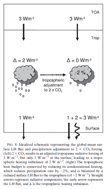
So, with the idea of an instantaneous doubling, if the surface increase in radiative forcing is less than the tropopause increase in radiative forcing, this must mean that the balance of energy is absorbed within the atmosphere. And also, we have to consider what happens as a result of the surface energy imbalance.

The numbers I use here are Ramanathan’s numbers from his 1981 paper. Later, and more accurate, numbers have been calculated but don’t affect the main points of this analysis. The reason for reviewing his analysis is because some (but not all) of the inherent responses of the climate system are explicitly calculated – making it easier to understand than the output of GCM.

Immediate Response

The immediate result of this doubling of CO2 is a reduced emission of radiation (OLR = outgoing longwave radiation) from the climate system into space. See the Atmospheric Radiation and the “Greenhouse” Effect series for detailed explanations of why.

At the tropopause the OLR reduces by 3.1 W/m², and downward emission from the stratosphere into the troposphere increases by 1.2 W/m².

This results in a net forcing at the tropopause of 4.3 W/m². Most of the radiation from the atmosphere to the surface (as a result of more CO2) is absorbed by water vapor. So at the surface the DLR (downward long radiation) increases by only 1.2 W/m² – this is the (immediate) surface forcing. Here is a simple graphical explanation of why the OLR decreases and the DLR increases:

Figure 2 – Click for a larger image

Response After a Few Months

The stratosphere cools and reaches a new radiative equilibrium. This reduces the downward emission from the stratosphere by a small amount. The new value of radiative forcing at the tropopause = 4.2 W/m².

Response After Many Decades

The surface-troposphere warms until a new equilibrium is reached – the radiative forcing at the tropopause has returned to zero.

The Surface

So let’s now consider the surface. Take a look at Figure 1 again. The values/ranges we will consider are calculated by a model. This doesn’t mean they are correct. It means that applying well-understood processes in a simplistic way gives us a “first order” result. The reason for assessing this kind of approach is because our mental models are usually less accurate than a calculated result which draws on well-understood physics.

As Ramanathan says in his 1998 paper:

As a caveat, the system we considered up to this point to elucidate the principles of warming is a highly simplified linear system. Its use is primarily educational and cannot be used to predict actual changes.

Process 1 is as already described – the surface forcing increases by just over 1 W/m². But the balance of 3 W/m² goes into heating the troposphere.

Process 2 – The warming of the troposphere results in increases downward radiation to the surface (because the hotter the body, the higher the radiation emitted). The calculated value is an additional 2.3 W/m², so the surface imbalance is now 3.5 W/m² and the surface temperature must increase in response. Upwards surface radiation and/or sensible and latent heat will increase to balance.

Process 3 – The surface emission of radiation increases at around 5.5 W/m² for every 1°C of surface temperature increase. But this is almost balanced by increased downward radiation from the atmosphere (“back radiation”). The net effect is only about 10% of the change in upward radiation. So latent heat and sensible heat increase to restore the energy balance, but this also heats the troposphere.

Process 4 – The tropospheric humidity increases. This increases the emissivity of the atmosphere near the surface, which increases the back radiation.

So essentially some cycles are reinforcing each other (=positive feedback). The question is about the value of the new equilibrium point.

From Ramanathan (1981)

Figure 3

In Ramanathan’s 1981 paper he gives some basic calculations before turning to GCM results. The basic calculations are quite interesting because one of the purposes of the paper was to explain why some model results of the day produced very small equilibrium temperature changes.

Sadly for some readers, a little maths is necessary to reproduce the result. It is simple maths because it is based on simple concepts – as already presented. As much as possible I follow the equation numbers and notations from Ramanathan’s 1981 paper.

Calculations

Energy balance at an “average” surface:

Upward flux = Downward flux

→ LH + SH + F↑ = F↓ + S + ΔR ….[2]

where LH = latent heat, SH = sensible heat, F↑ = surface emitted upward radiation, F↓ = surface downward radiation from the atmosphere, S = solar radiation absorbed, ΔR = instantaneous change in energy absorbed at the surface due to an increase in CO2

And see note 1. We have simple formulas for the left hand side.

F↑ = σT⁴….[3a]

Latent heat and sensible heat flux have “bulk aerodynamic formulas” (note 2):

LH = ρLC_DV (q*_M – q_S) ….[3b]

SH = ρc_pC_DV (T_M – T_S) ….[3c]

Where ρ = density of air = 1.3 kg/m, L = latent heat of water vapor = 2.5 x 10⁶, C_D = empirically determined coefficient ≈ 1.3 x10^-3, V = average wind speed at some reference height above the surface ≈ 5 m/s, q*_M = specific humidity at saturation at the surface temperature of the ocean, q_S = specific humidity at the reference height, T_M = temperature of the ocean at the surface, T_S = temperature of the air at the reference height (typically 10m).

To give an idea of typical values, for every 1°C difference between the surface and the air at the reference height, SH = 8.5 W/m²K, and with a relative humidity of 80% at the reference height (and 100% at the ocean surface), LH = 55 W/m²K.

Now we consider changes.

T_M‘ is the change in the surface temperature of the ocean as the result of the increased CO2, and similar notation for other changes in values. Missing out a few steps that you can read in the paper:

T_M‘ = ΔR(0) + ΔF↓(2) + ΔF↓(3) ….[13]

[ ∂LH/∂T_M + ∂SH/∂T_M + 4σT_M³] + [ ∂LH/∂T_S + ∂SH/∂T_S ].T_S‘/T_M‘

This probably seems a little daunting to a lot of readers.. so let’s explain it:

The parameter on the top line in black, ΔR(0) is the surface radiative forcing from the increase in CO2
The red terms are the changes in downward radiation as a result of process 2 and 3 described above
The blue terms are the changes in upward flux due to only the ocean surface temperature changing
The green terms are the changes in upward flux due to only the atmospheric temperature near the surface changing
The blue term ≈ 30 W/m²K @ 15°C; the green term ≈ -8.5 W/m²K @ 15°C (note 3)

And the smaller the total under the line, the higher the increase in temperature. And there are two competing terms:

As the surface temperature of the ocean increases the heat transfer from the ocean to the atmosphere increases
As the atmospheric temperature (just above the ocean surface) increases the heat transfer from the ocean to the atmosphere decreases

As an interesting comparison, Ramanathan reviewed the methods and results of Newell & Dopplick (1979) who found a changed surface temperature, Tm’ = 0.04 °C as a result of CO2 doubling. Effectively, very little change in surface temperature as a result of doubling of CO2.

Ramanathan states that the calculations of Newell & Dopplick had ignored the red terms and the green terms. Ignoring the red terms means that the heating of the atmosphere is ignored. Ignoring the green terms means that the effect of the ocean surface heating is inflated – if the ocean surface heats and the atmosphere just above somehow stayed the same then the heat transferred would be higher than if the atmospheric temperature also increased as a result. (Because heat transfer depends on temperature difference).

I expect that many people doing their own estimates will be working from similar assumptions.

Later Work

Here is a graphic from Andrews et al (2009), reference and free link below, which shows the simplified idea:

From Andrews et al (2009)

Figure 4

The paper itself is well worth reading and perhaps will be the subject of another article at a later date.

Conclusion

I haven’t demonstrated that the surface will warm by 3°C for a doubling of CO2. But I hope I have demonstrated the complexity of the processes involved and why a simplistic calculation of how the surface responds immediately to the surface forcing is not the complete answer. It is nowhere near the complete answer.

The surface temperature change as a result of doubling of CO2 is, of course, a massively important question to answer. GCM’s are necessarily involved despite their limitations.

Re-iterating what Ramanathan said in his 1998 paper in case anyone thinks I am making a case for a 3°C surface temperature increase:

As a caveat, the system we considered up to this point to elucidate the principles of warming is a highly simplified linear system. Its use is primarily educational and cannot be used to predict actual changes.

References

Trace Gas Greenhouse Effect and Global Warming, V. Ramanathan, Ambio (1998)

The role of ocean-atmosphere interactions in the CO2 climate problem, V Ramanathan, Journal of Atmospheric Sciences (1981)

Thermal equilibrium of the atmosphere with a given distribution of atmospheric humidity, Manabe & Wetherald, Journal of Atmospheric Sciences (1967)

A Surface Energy Perspective on Climate Change, Andrews, Forster & Gregory, Journal of Climate (2009)

Notes

Note 1: The equation ignores the transfer of heat into the ocean depths

Note 2: The “bulk aerodynamic formulas” – as they have become known – are more usable versions of the fundamental equations of heat and water vapor flux. Upward sensible heat flux, SH = ρc_p<wT>, where w = vertical velocity, T = temperature, so <wT> is the time average of the product of vertical velocity and temperature. However, turbulent motions are so rapid, changing on such short time intervals that measurement of these values is usually impossible (or requires intensive measurement with specialist equipment in one location). We can write,

w = <w> + w’, where <w> = mean vertical velocity and w’ = deviation of vertical velocity from the mean, likewise T = <T> + T’.

So:

<wT> = <w><T> + <w’ T’> or, Total = Mean + Eddy

Near the surface the mean vertical motion is very small compared with the turbulent vertical velocity and so the turbulent component, <w’ T’>, dominates. Therefore,

SH = c_pρ <w’ T’>

LH = L ρ <w’ T’>

where c_p= specific heat capacity of air, ρ = density of air, L = latent heat of water vapor

By various thermodynamic arguments, and especially by lots of empirical measurements, an estimate of heat transfer can be made via the bulk aerodynamic formulas shown above, which use the average horizontal wind speed at the surface in conjunction with the coefficients of heat transfer, which are related to the friction term for the wind at the ocean surface.

Note 3: The calculation of each of the partial derivative terms is not shown in the paper, these are my calculations. I believe that ∂LH/∂T_S = 0, most of the time – this is because if the atmosphere at the reference height is not saturated then an increase in the atmospheric temperature, T_S, does not change the moisture flux, and therefore, does not change the latent heat. I might be wrong about this, and clearly some of the time this assumption I have made is not valid.

Posted in Atmospheric Physics, Basic Science | 184 Comments »

« Newer Posts - Older Posts »

	. on The Amazing Case of “Bac…
	pjmacha on Extreme Weather #17 – Mo…
	E. Schaffer on Clouds & Water Vapor – Par…
	E. Schaffer on Clouds & Water Vapor – Par…
	Rok Adamlje on Clouds and Water Vapor –…
	Everything You Need… on Sensible Heat, Latent Heat and…
	Philip Schmidt on The “Greenhouse” E…
	Philip Schmidt on The Real Second Law of Th…
	Barton Paul Levenson on Opinions and Perspectives…
	Your Guide to Gambli… on Natural Variability and Chaos…
	Mane Oliva on The Amazing Case of “Bac…
	Tucker C on Heat Transfer Basics – P…
	Alll Teens Relate on Stratospheric Cooling
	DeWitt Payne on Clouds & Water Vapor – Par…
	DeWitt Payne on The Imaginary Second Law of…

Evaluating and Explaining Climate Science

My Prediction

My Challenge

The Usual Caveat

My Second Prediction

Coriolis

Some Maths

Geostrophic Balance and the Magnitude of the Coriolis Effect

Conclusion

Notes

Goody & Yung’s Big Mistake

Kepler & Milankovitch

Energy Conversion in the Atmosphere & at the Surface

The Gulags for Everyone? – Climatology Loses Its Rational Basis

The Main Point

Dodging the Bullet

Conclusion

Notes

Eddy Diffusivity

Measurements of Eddy Diffusivity

Eddy Diffusivity and Buoyancy Gradient

Modeling, Non-Linearity and Climate Sensitivity Measurement Problems

Simple Models

Conclusion

Articles in this Series

References

Notes

The Simple Model of Climate Sensitivity

Real Life Ocean Mixed Layer

How Deep is the Ocean Mixed Layer?

Trying Simple Models with Varying MLD

Non-Linearity

Losing the Plot?

The Next Phase – More Realistic Ocean Model

Conclusion

Articles in this Series

References

Climate Sensitivity Is All About Feedback

Theory and Measurement

Regression

Simulations

Discussion of Results

Maths

Murphy & Forster 2010

Linear Feedback Relationship?

Conclusion

Articles in this Series

References

Notes

Immediate Response

Response After a Few Months

Response After Many Decades

The Surface

Calculations

Later Work

Conclusion

References

Notes

Pages

Recent Posts

Recent Comments

Categories

Climate Websites

Science of Doom Key Pages

Subscribe by RSS

Subscribe by Email

Archives

Meta