Recap
Part One of the series introduced the shortwave radiation from the sun, the balancing longwave radiation from the earth and the absorption of some of that longwave radiation by various “greenhouse” gases. The earth would be a cold place without the “greenhouse” gases.
Part Two discussed the factors that determine the relative importance of the various gases in the atmosphere.
Part Three and Four got a little more technical – an unfortunate necessity. Part Three introduced Radiative Transfer Equations including the Beer-Lambert Law of absorption. It also introduced the important missing element in many people’s understanding of the role of CO2 – re-emission of radiation as the atmosphere heats up.
Part Four brought in band models. These are equations which quite closely match the real absorption of CO2 (and the other greenhouse gases) as a function of wavelength. They aren’t strictly necessary to get to the final result, but they have an important benefit – they allow us to easily see how the absorption changes as the amount of gas increases. And they are widely used in climate models because they reduce the massive computation time that are otherwise involved in solving the Radiative Transfer Equations. The important outcome as far as CO2 is concerned – “saturation” can be technically described.
Solving the Equations
The equations of absorption and radiation in the atmosphere – the Radiative Transfer Equations – have been known for more than 60 years. Solving the equations is a little more tricky.
Like many real world problems, the radiative processes in the atmosphere can be mathematically described from 1st principles but not “analytically” solved. This simply means that numerical methods have to be used to find the solution.
There’s nothing unproven or “suspicious” about this approach. Every problem from stresses in bridges and buildings to heat dissipation in an electronic product uses this method.
The problem of the effect of greenhouse gases in the atmosphere is formulated with a 1-dimensional model. This is the simplest approach (after the “billiard ball” model we saw in part one). But like any model there are certain assumptions that have to be made – the boundary conditions. And over the last 40 years different scientists have approached the problem from slightly different directions, making comparisons not always easy.
Because the role of CO2 in the atmosphere is causing such concern the results of these models is consequently much more important. And so a lot of effort recently has gone into standardizing the approach. We’ll look at a few results, but first, for those who would like to visualize what modern methods of “numerical analysis” are about – a little digression.. (and for those who don’t, jump ahead to the Ramanathan.. subheading).
Digression on Numerical Methods

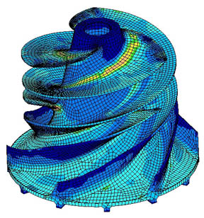
Stress analysis in an impeller
Here’s a visualization of “finite element analysis” of stresses in an impeller. See the “wire frame” look, as if the impeller has been created from lots of tiny pieces?
In this totally different application, the problem of calculating the mechanical stresses in the unit is that the “boundary conditions” – the strange shape – make solving the equations by the usual methods of re-arranging and substitution impossible. Instead what happens is the strange shape is turned into lots of little cubes. Now the equations for the stresses in each little cube are easy to calculate. So you end up with 1000’s of “simultaneous” equations. Each cube is next to another cube and so the stress on each common boundary is the same. The computer program uses some clever maths and lots of iterations to eventually find the solution to the 1000’s of equations that satisfy the “boundary conditions”.
In the case of the radiative transfer equations (RTE) we want to know the temperature profile up through the atmosphere. The atmosphere is divided into lots of thin slices. Each “slice” has some properties attached to it:
- gases like water vapor, CO2, CH4 at various concentrations with known absorption characteristics for each wavelength
- a temperature -unknown – this is what we want to find out
- radiation flowing up and down through the “slice” at each wavelength – unknown – we also want to find this out
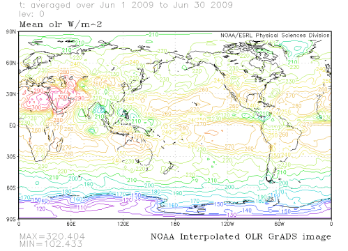
And we have important boundary conditions – like the OLR (outgoing longwave radiation) at the top of the atmosphere. We know this is about 239 W/m2 (see The Earth’s Energy Budget – Part One). Using the boundary conditions, we solve the radiative transfer equations for each slice, and the computer program does this by creating lot of simultaneous equations (energy in each wavelength flowing between each slice is conserved).
Ramathan and Coakley, 1978
Why bring up an old paper? Partly to demonstrate some of the major issues and one interesting approach to solving them, but also to give a sense of history. A lot of people think that the concern over greenhouse gases is something new and perhaps all to do with the IPCC or Al Gore.
Back in 1978, V. Ramanathan and J.A. Coakley’s paper Climate Modeling through Radiative-Convective Models was published in Reviews of Geophysics and Space Physics.
It wasn’t the first to tackle the subject and points to the work done by Manabe and Strickler in 1964. By the way, V. Ramanathan is a bit of a trooper, having published 169 peer-reviewed papers in the field of atmospheric physics from 1972-2009..
I’m going to call the paper R&C – so R&C cover the detailed maths of course, but then discuss how to deal with the “problem” of convection.
In the lower part of the atmosphere heat primarily moves through convection. Hot air rises – and consequently moves heat. Radiation also transfers heat but less effectively. The last section of Part Three introduced this concept with the “gray model”. Here was the image presented:

The Gray Model of Radiative Equilibrium, from "Handbook of Atmospheric Science" Hewitt and Jackson (2003)
Remember that each section of the atmosphere radiates energy according to its temperature. So when we are solving the equations that link each “slice” of the atmosphere we have to have a term for temperature.
But how do we include convection? If we don’t include it our analysis will be wrong but solving for convection is a very different kind of problem, related to fluid dynamics..
What R&C did was to approach the numerical solution by saying that if the energy transfer from radiation at any point in their vertical profile resulted in a temperature gradient less than that from convection then use the known temperature profile at that point. And if it was greater than the temperature gradient from convection then we don’t have to think about convection in this “slice” of the atmosphere.
By the way, the terminology around how temperature falls with height through the atmosphere is called “the lapse rate” and it is about 6.5K/km.
These assumptions in the two cases didn’t mean that absorption and re-radiation were ignored in the lower part of the atmosphere – not at all. But the equations can’t be solved without including temperature. The question is, do we solve the equations by calculating temperature – or do we use an “externally imposed” temperature profile?
There is lots to digest in the paper as it is a comprehensive review. The few of interest for this post:
Doubling CO2 from 300ppm to 600ppm
- Longwave radiative forcing at the top of the troposphere – 3.9W/m2
- Surface temperature increase 1.2°C
- Result of change in radiative forcing when relative humidity stays constant (rather than absolute humidity staying constant) – surface temperature increase is doubled
(Note: this is not quite the “standardized” version of doubling considered today of 287ppm – 576ppm)
Relative Effect of CO2 and water vapor
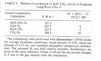
This is under 1978 conditions of 330ppmv for CO2 and in a cloudy sky. Here they run the calculation with and without different gases and look at how much more outgoing longwave radiation there is, i.e. how much longwave radiation is absorbed by each gas. The problem is complicated by the fact that there is an overlap in various bands so there are combined effects.
- Removing CO2 (and keeping water vapor) – 9% increase in outgoing flux
- Removing water vapor (and keeping CO2) – 25% increase in outgoing flux
Everyone (= lots of people in lots of websites who probably know a lot more than me) says that this paper calculates the role of CO2 between 9% and 25% but that’s not how I read it. Perhaps I missed something.

Extract from Ramanathan & Coakley (1978) - Relative contribution of H2O, CO2 and O3
What it says to me is that overlap must be significant because if we take out water vapor it is only a 25% effect. And if we take out CO2 it is a 9% effect. (I have emailed the great V. Ramanathan to ask this question, but have not had a response so far.)
Therefore, guessing at the overlap effect, or more accurately, assigning the overlap equally between the two, water vapor has about 2.5 times the effect of CO2. As you will see in the next paper, this is about what our later results show.
So, more than 30 years ago, atmospheric physicists calculated some useful results which have been confirmed and refined by later scientists in the field.
Kiehl and Trenberth 1997
Earth’s Annual Global Mean Energy Budget by J.T.Kiehl and Kevin Trenberth was published in Bulletin of the American Meteorological Society in 1997. (The paper is currently available from this link)
The paper is very much worth a read in its own right as it reviews and updates the data at the time on the absorption and reflection of solar radiation and the emission and re-absorption of longwave radiation. (There is an updated paper – that free link currently works – in 2008 but it assumes the knowledge of the 1997 paper so the 1997 paper is the one to read).
This paper doesn’t assess the increase in radiative forcing or the consequent temperature change that might imply from the current levels of CO2, CH4 etc. Instead this paper is focused on separating out the different contributions to shortwave and longwave absorbed and reflected and so on.
What is interesting about this paper for our purposes in that they quantify the relative role of CO2 and water vapor in clear sky and cloudy sky conditions.
To do the calculation of absorption and re-emission of longwave radiation they used the US Standard Atmosphere 1976 for vertical profiles of temperature, water vapor and ozone. They assumed 353ppmv of CO2, 1.72ppmv of CH4 and 0.31 of N2O, all well mixed. Note that, like R&C, they assumed a temperature profile to carry out the calculations because convection dominates heat movement in the lower part of the atmosphere.
Two situations are considered in their calculations – clear sky and cloudy sky.
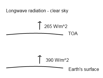
Let’s look at the clear sky results:

Upward Longwave Radiation, Numbers from Kiehl & Trenberth (1997)
The radiation value from the earth’s surface matches the temperature of 288K (15°C) – you can see how temperature and radiation emitted are linked in the maths section at the end of CO2 – An Insignificant Trace Gas? Part One.
The value calculated initially at the top of atmosphere was 262 W/m2, the value was brought into line with the ERBE measured value of 265 W/m2 by a slight change to the water vapor profile, see Note 1 at the end.
Of course, the difference between the surface and top of atmosphere values is accounted for by absorption of long wave radiation by water vapor, CO2, etc. No surprise to those who have followed the series to this point.
By comparison the cloudy sky numbers were:
- Surface – 390W/m2 (no surprise, the same 288K surface)
- TOA – 235W/m2. More radiation is absorbed when clouds are present. See Note 2 at end.
Now onto the important question: of the 125W/m2 “clear sky greenhouse effect”, what is the relative contribution of each atmospheric absorber?
The only way to calculate this is to remove each gas in turn from the model and recalculate.
Clear Sky
- Water vapor contributes 75W/m2 or 60% of the total
- CO2 contributes 32W/m2 or 26% of the total
Cloudy Sky
- Water vapor contributes 51W/m2 or 59% of the total
- CO2 contributes 24W/m2 or 28% of the total
Note that significant longwave radiation is also absorbed by liquid water in clouds.
Conclusion
Using these three elements:
- the well known equations of radiative transfer (basic physics)
- the measured absorption profiles of each gas
- the actual vertical profiles of temperature and concentrations of the various gases in the atmosphere
The equations can be solved in a 1-d vertical column through the atmosphere and the relative effects of different gases can be separated out and understood.
Additionally, the effect in “radiative forcing” of the current level of CO2 and of CO2 doubling (compared with pre-industrial levels) can be calculated.
This radiative forcing can be applied to work out the change in surface temperature – with “all other things being equal”.
“All other things being equal” is the way science progresses – you have find a way to separate out different phenomena and isolate their effects.
The temperature increase in the R&C paper of 1.2°C only tells us the kind of impact from this level of radiative forcing. Not what actually happens in practice, because in practice we have so many other factors affecting our climate. That doesn’t mean it isn’t a very valuable result.
Now the value of radiative forcing will be slightly changed if “all other things are not equal” but if the concentration of water vapor, CO2, CH4, etc are similar to our model the changes will not be particularly significant. It is only really the actual temperature profile through the atmosphere that can change the results. This is affected by the real climate of 3d effects – colder or warmer air blowing in, for example. Overall, from comparing the results of 3-d models – ie the average results of lots of 1-d models, the values are not significantly changed – more on this in a later post.
We see that CO2 is around 25% of the “greenhouse” effect, with water vapor at around 60%.
Note that the calculation uses the “US Standard Atmosphere” – different water vapor concentrations will have a significant impact, but this is an “averaged” profile.
The only way to really determine the numbers is to run the RTE (radiative transfer equations) through a numerical analysis and then redo the calculations without each gas.
The two questions to ask if you see very different numbers is “under what conditions?” and more importantly “how did you calculate these numbers?” Hopefully, for everyone following the series it will be clear that you can’t just eyeball the spectral absorption and the average relative concentrations of the gases and tap it out on a calculator.
I thought it would be all over by Part Three, but CO2 is a gift that keeps on giving..
Updates:
CO2 – An Insignificant Trace Gas? Part Six – Visualization
CO2 – An Insignificant Trace Gas? Part Seven – The Boring Numbers
CO2 – An Insignificant Trace Gas? – Part Eight – Saturation
See also – Theory and Experiment – Atmospheric Radiation – demonstrating the accuracy of the radiative-convective model from experimental results
Notes and References
Note 1 – As Kiehl and Trenberth explain, there are some gaps in our knowledge in a few places of exactly how much energy is absorbed or reflected from different components under different conditions. One of the first points that they make is that the measurement of incoming shortwave and outgoing longwave (OLR) are still subject to some questions as to absolute values. For example, the difference between incoming solar and the ERBE measurement of OLR is 3W/m2. There are some questions over the OLR under clear sky conditions. But for the purposes of “balancing the budget” a few numbers are brought into line as the differences are still within instrument uncertainty.
Note 2 – I didn’t want to over-complicate this post. Cloudy sky conditions are more complex. Compared with clear skies clouds reflect lots of solar (shortwave) radiation, absorb slightly more solar radiation and also absorb more longwave radiation. Overall clouds cool our climate.
References
Climate Modeling through Radiative-Convective Models , V. Ramanathan and J.A. Coakley, Reviews of Geophysics and Space Physics (1978)
Earth’s Annual Global Mean Energy Budget , J.T.Kiehl and Kevin Trenberth, Bulletin of the American Meteorological Society (1997)
Read Full Post »
