The Science of Doom

If you look at model outputs for rainfall in the last IPCC report, or in most papers, it’s difficult to get a feel for what models produce, how they compare with each other, and how they compare with observational data. It’s common to just show the median of all models.

In this, and some subsequent articles, I’ll try and provide some level of detail.

Here are some comparisons from a set of models from the Max Planck Institute for Meteorology. MPI is just one of about 20 climate modeling centers around the world. They took part in the Climate Model Intercomparison Project (CMIP5). As part of that project, for the IPCC 5th assessment report (AR5), they ran a number of simulations. Details of CMIP5 in the Taylor et al reference below.

Future scenarios vs modeled history

Here is the % change in rainfall – 2081-2100 vs 1979-2005 from one of the MPI models (MPI-ESM-LR) for 3 scenarios. The median of 3 runs for each scenario is compared with the median of 3 runs for the historical period, and we see the % change:

Figure 1 – Simulations from MPI-ESM-LR for 3 RCPs vs simulation of historical – Click to expand

The scenarios (Representative Concentration Pathways) in brief (and see van Vuuren reference below):

• rcp2.6 – large reductions in CO2 emissions within a short space of time. Conceptual model – shutting off the world’s power stations, and no burning of fossil fuels, by 2030
• rcp 4.5 – substantial improvements in reducing CO2 emissions
• rcp 6 – not shown as they didn’t model it. This is probably roughly where we will be in 2100 based on current trends
• rcp 8.5 – extreme CO2 emissions, often misleadingly cited as “business as usual” (see Opinions and Perspectives – 3 – How much CO2 will there be? And Activists in Disguise and Opinions and Perspectives – 3.5 – Follow up to “How much CO2 will there be?”)

We can see that rcp 2.6 has some small reductions in rainfall in northern Africa, Middle East and a few other regions. RCP 8.5 has large areas of greatly reduced rainfall in northern Africa, Middle East , SW Africa, the Amazon, and SW Australia.

So from a model only point of view the less emissions the better.

It’s common to find that RCP6 is not modeled, something that I find difficult to understand. I understand that computing time is valuable but RCP6 seems like the emissions pathway we are currently on.

Perhaps it should be explicitly stated that the simulation results of RCP4.5 and RCP6 are effectively identical – if that is in fact the case. That by itself would be useful information given that there is a substantial difference in CO2 emissions between them.

I had a look at a couple of regions of interest – Australia:

Figure 2 – Australia – Simulations from MPI-ESM-LR for 3 RCPs vs simulation of historical – Click to expand

And Europe:

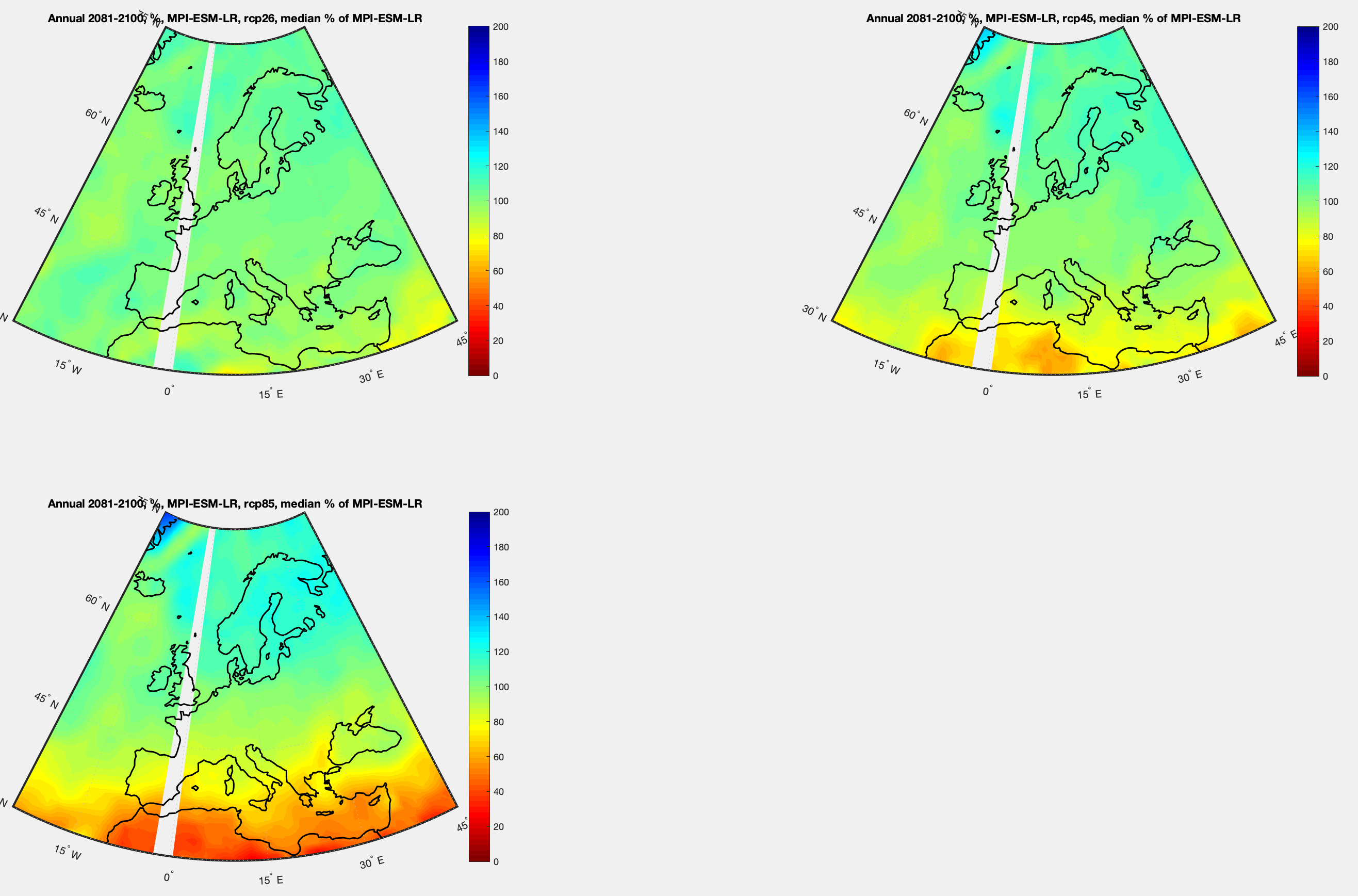
Figure 3 – Europe – Simulations from MPI-ESM-LR for 3 RCPs vs simulation of historical – Click to expand

Modeled History vs Observational History

Here we compare the historical MPI model runs with observations (GPCC). MPI has 3 models and a total of 8 runs:

• MPI-ESM-LR (3 simulations)
• MPI-ESM-MR (3 simulations)
• MPI-ESM-P (2 simulations)

Each model that takes part in CMIP5 produces one or more simulations over identical ‘historical’ conditions (our best estimate of them) from 1850-2005.

I compared the median of each model with GPCC over the last 27 years of the ‘historical’ period, 1979-2005:

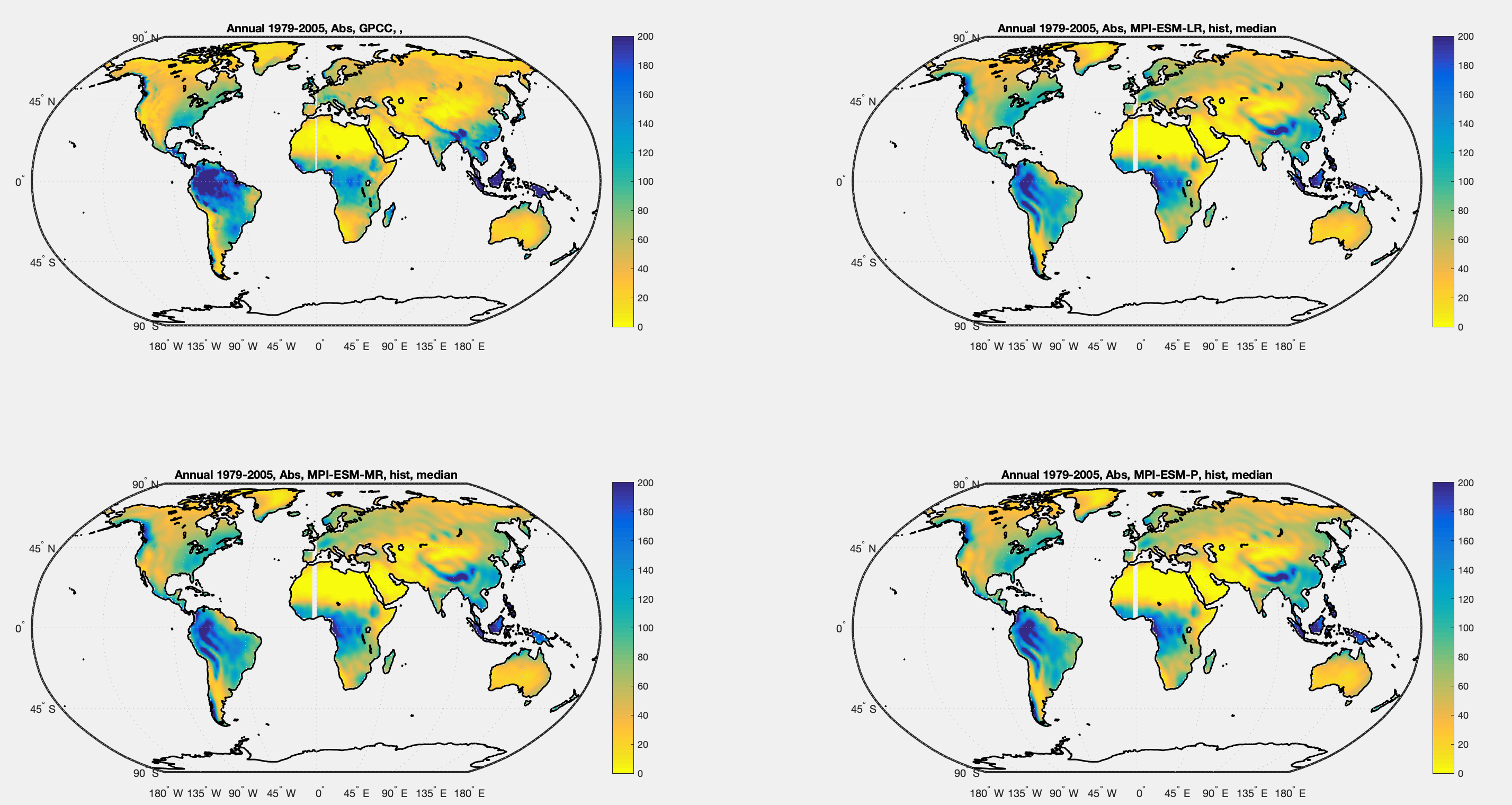
Figure 4 – The median of simulations from each MPI model vs observation 1979-2005 – Click to expand

And the % difference of each MPI model vs GPCC over the same period:

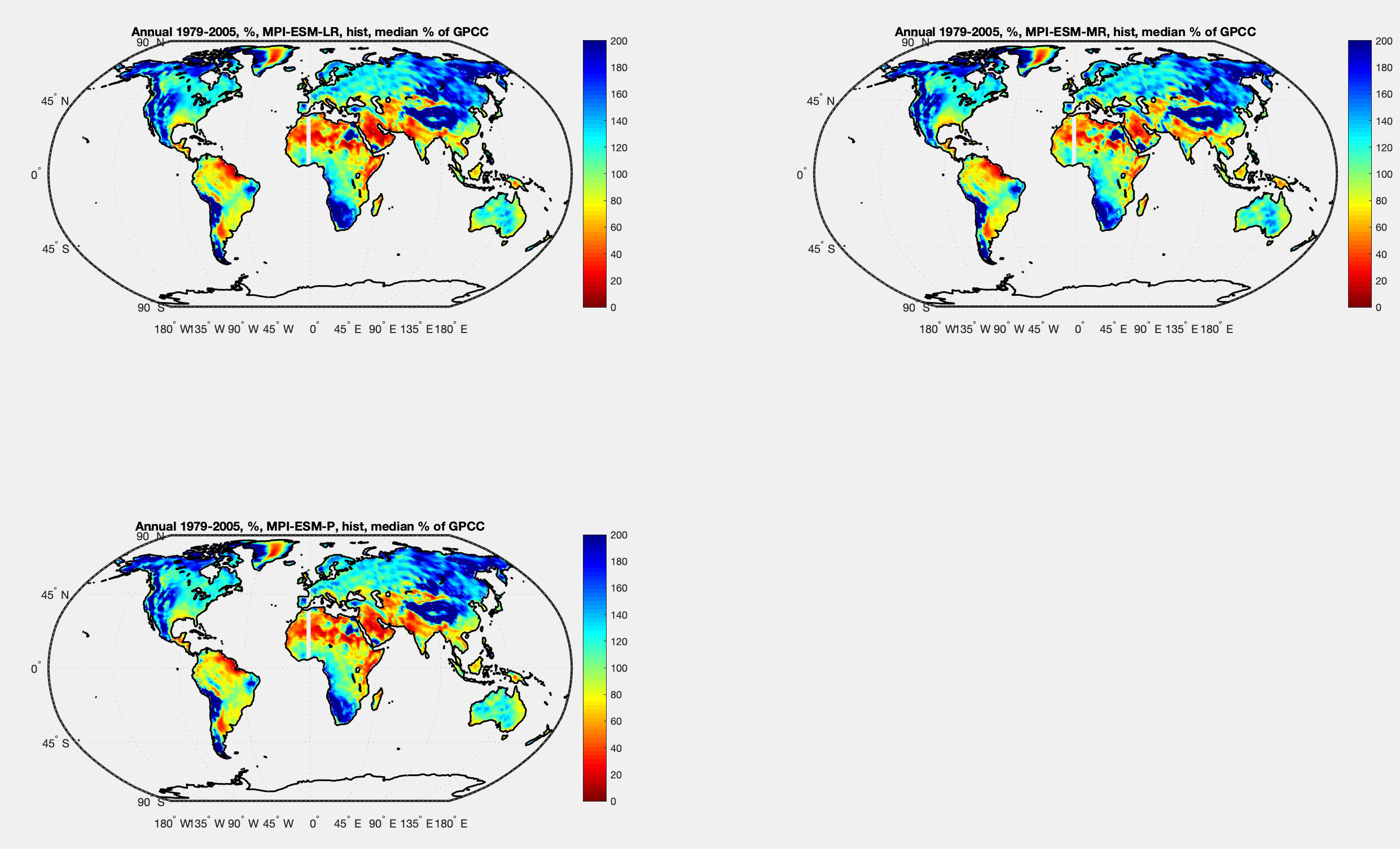
Figure 5 – The median of simulations from each MPI model, % change over observation 1979-2005 – Click to expand

The different models appear quite similar. So let’s take the median of all 8 runs across the 3 models and compare with observations (GPCC) for clarity (the graph title isn’t quite correct, this is across the 3 models):

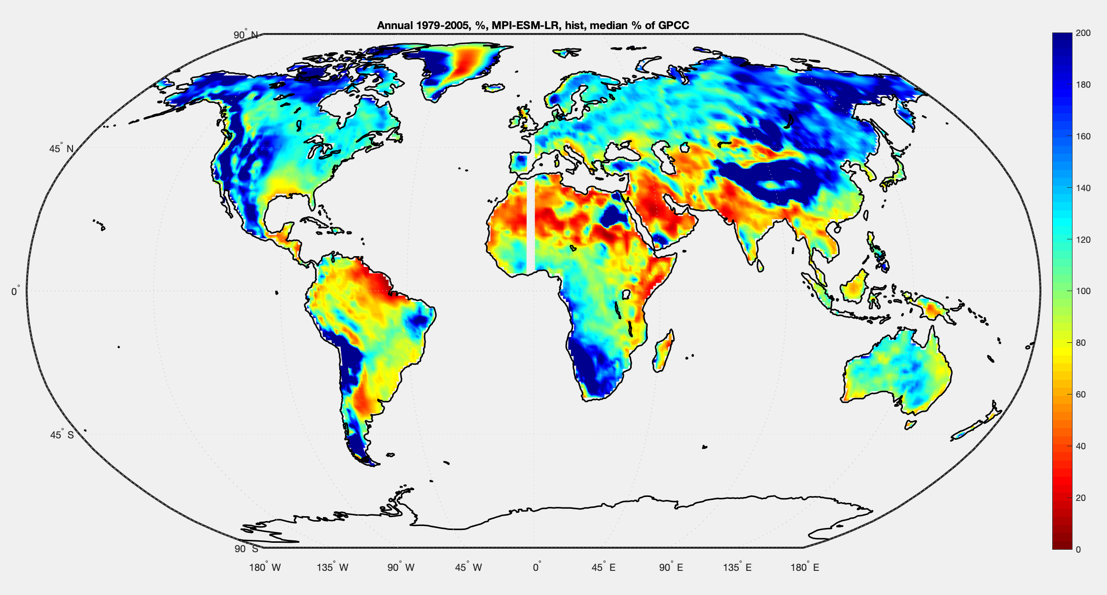
Figure 6 – The median of simulations from all MPI models, % change over observation 1979-2005 – Click to expand

The same, highlighting Australia:

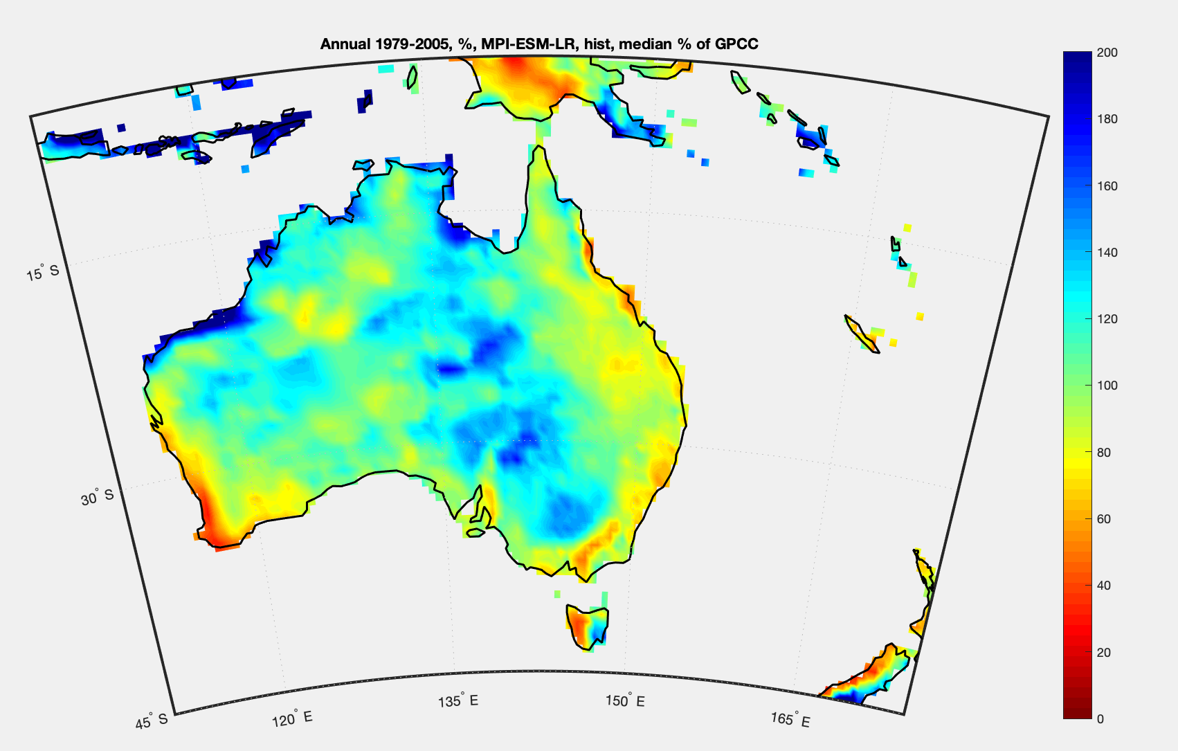
Figure 7 – Australia – median of simulations from all MPI models, % change over observation 1979-2005 – Click to expand

And highlighting Europe:

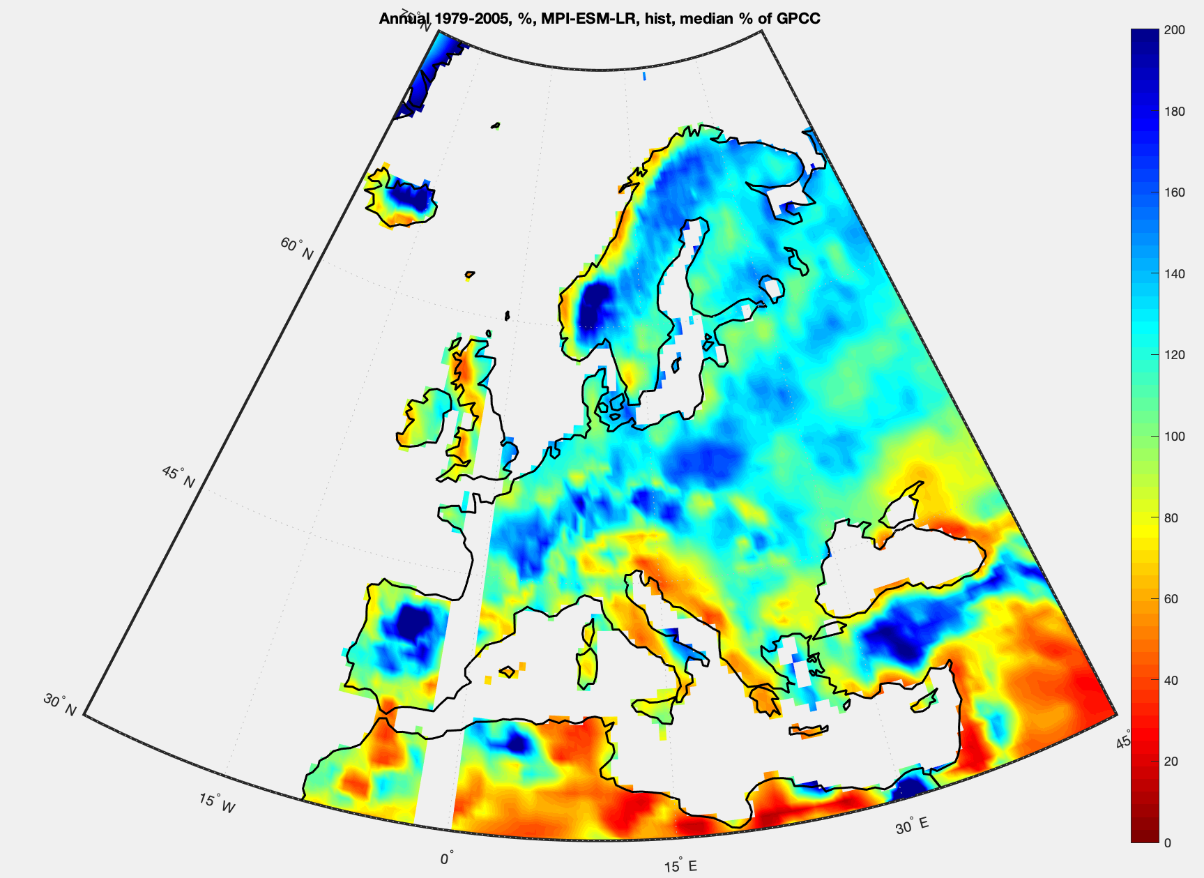
Figure 8 – Europe – median of simulations from all MPI models, % change over observation 1979-2005 – Click to expand

I’m not trying to draw any big conclusions here, more interested in showing what model results look like.

But the one thing that stands out in a first look, at least to me – the difference between the MPI model and observations (over the same time period) is more substantial than the difference between the MPI model for 2080-2100 and the MPI model for recent history, even for an extreme CO2 scenario (RCP8.5).

If you want to draw conclusions from a climate model on rainfall, should you compare the future simulations with the simulation of the recent past? Or future simulations with actual observations? Or should you compare past simulations with actual and then decide whether to compare future simulations with anything?

References

An overview of CMIP5 and the experiment design, Taylor, Stouffer & Meehl, AMS (2012)

GPCP data provided by the NOAA/OAR/ESRL PSL, Boulder, Colorado, USA, from their Web site at https://psl.noaa.gov/

GPCC data provided from https://psl.noaa.gov/data/gridded/data.gpcc.html

CMIP5 data provided by the portal at https://esgf-data.dkrz.de/search/cmip5-dkrz/

The representative concentration pathways: an overview, van Vuuren et al, Climatic Change (2011)